DSLWP-B has now been for more than a month in lunar orbit, since the orbital injection was made on May 25. Scott Tilley VE7TIL has sent me his latest batch of S-band Doppler measurements, including data for all this first lunar month. Having a complete lunar month of data is interesting for orbit determination purposes, since it gives observability of the orbit from all possible right ascension angles.
I have run my orbit determination with the new data.
Category: Space
Spacecraft and space science
DSLWP-B GMSK detector
Following the success of my JT4G detector, which I used to detect very weak signals from DSWLP-B and was also tested by other people, I have made a similar detector for the 250baud GMSK telemetry transmissions.
The coding used by the DSLWP-B GMSK telemetry follows the CCSDS standards for turbo-encoded GMSK/OQPSK. The relevant documentation can be found in the TM Synchronization and Channel Coding and Radio Frequency and Modulation Systems–Part 1: Earth Stations and Spacecraft blue books.
The CCSDS standards specify that a 64bit ASM shall be attached to each \(r=1/2\) turbo codeword. The idea of this algorithm is to correlate against the ASM (adequately precoded and modulated in GMSK). The ASM spans 256ms and the correlation is done as a single coherent integration. As a rule of thumb, this should achieve a reliable detection of signals down to around 12dB C/N0, which is equivalent to -12dB Eb/N0 or -22dB SNR in 2500Hz. Note that the decoding threshold for the \(r=1/2\) turbo code is around 1.5dB Eb/N0, so it is much easier to detect the GMSK beacon using this algorithm than to decode it. The difficulty of GMSK detection is comparable to the difficulty of JT4G decoding, which has a decoding threshold of around -23dB SNR in 2500Hz.
Here I explain the details of this GMSK ASM detector. The Python script for the detector is dslwp_gmsk.py.
DSLWP-B detected with 7 element yagi
Yesterday I tried to detect DSLWP-B using my 7 element Arrow satellite yagi. The test schedule for DSLWP-B was as follows: active between 21:00 and 23:00 UTC on 2018-06-22. GMSK telemetry transmitted both on 435.4MHz and 436.4MHz. JT4G only on 435.4MHz every 10 minutes starting at 21:10. The idea was to record the tests with my equipment and the run my JT4G detector, which should be able to detect very weak signals. Today I have processed the recorded data and I have obtained a clear detection of one of the JT4G transmissions (albeit with a small SNR margin). This shows that it is possible to detect DSLWP-B with very modest equipment.
DSLWP-B first JT4G test
Yesterday, between 9:00 and 11:00, DSLWP-B made its first JT4G 70cm transmissions from lunar orbit. Several stations such as Cees Bassa and the rest of the PI9CAM team at Dwingeloo, the Netherlands, Fer IW1DTU in Italy, Tetsu JA0CAW and Yasuo JA5BLZ in Japan, Mike DK3WN in Germany, Jiang Lei BG6LQV in China, Dave G4RGK in the UK, and others exchanged reception reports on Twitter. Some of them have also shared their recordings of the signals.
Last week I presented a JT4G detection algorithm intended to detect very weak signals from DSLWP-B, down to -25dB SNR in 2500Hz. I have now processed the recordings of yesterday’s transmissions with this algorithm and here I look at the results. I have also made a Python script with the algorithm so that people can process their recordings easily. Instructions are included in this post.
First results of DSLWP-B Amateur VLBI
In March this year I spoke about the Amateur VLBI with LilacSat-2 experiment. This experiment consisted of a GPS-synchronized recording of LilacSat-2 at groundstations in Harbin and Chongqing, China, which are 2500km apart. The experiment was a preparation for the Amateur VLBI project with the DSLWP lunar orbiting satellites, and I contributed with some signal processing techniques for VLBI.
As you may know, the DSLWP-B satellite is now orbiting the Moon since May 25 and the first Amateur VLBI session was performed last Sunday. The groundstations at Shahe in Beijing, China, and Dwingeloo in the Netherlands performed a GPS-synchronized recording of the 70cm signals from DSLWP-B from 04:20 to 5:40 UTC on 2018-06-10. I have adapted my VLBI correlation algorithms and processed these recordings. Here are my first results.
JT4G detection algorithm for DSLWP-B
Now that DSLWP-B has already been for 17 days in lunar orbit, there have been several tests of the 70cm Amateur Radio payload, using 250bps GMSK with an r=1/2 turbo code. Several stations have received and decoded these transmissions successfully, ranging from the 25m radiotelescope at PI9CAM in Dwingeloo, the Netherlands (see recordings here) and the old 12m Inmarsat C-band dish in Shahe, Beijing, to much more modest stations such as DK3WN‘s, with a 15.4dBic 20-element crossed yagi in RHCP. The notices for future tests are published in Wei Mingchuan BG2BHC’s twitter account.
As far as I know, there have been no tests using JT4G yet. According to the documentation of WSJT-X 1.9.0, JT4G can be decoded down to -17dB SNR measured in 2.5kHz bandwidth. However, if we don’t insist on decoding the data, but only detecting the signal, much weaker signals can be detected. The algorithm presented here achieves reliable detections down to about -25dB SNR, or 9dB C/N0.
This possibility is very interesting, because it enables very modest stations to detect signals from DSLWP-B. In comparison, the r=1/2 turbo code can achieve decodes down to 1dB Eb/N0, or 25dB C/N0. In theory, this makes detection of JT4G signals 16dB easier than decoding the GMSK telemetry. Thus, very small stations should be able to detect JT4G signals from DSLWP-B.
Update on DSLWP-B orbit determination
Last Sunday, I used Scott Tilley VE7TIL’s Doppler measurements of the DSLWP-B S-band beacon to perform orbit determination using GMAT. Yesterday Scott sent me the Doppler data he has been collecting during this week. I have re-run my orbit determination process to include this new data.
Below I show the Keplerian state that was determined on 2018-06-03, in comparison with the new state determined on 2018-06-10 (both are referenced to the same epoch of 2018-05-26 00:00:00 UTC).
% 20180603
%DSLWP_B.SMA = 8761.0758581
%DSLWP_B.ECC = 0.768016853537
%DSLWP_B.INC = 16.9728174682
%DSLWP_B.RAAN = 295.670653562
%DSLWP_B.AOP = 130.427472407
%DSLWP_B.TA = 178.126596496

% 20180610
DSLWP_B.SMA = 8762.40279943
DSLWP_B.ECC = 0.764697135746
DSLWP_B.INC = 18.6101083906
DSLWP_B.RAAN = 297.248156986
DSLWP_B.AOP = 130.40460851
DSLWP_B.TA = 178.09494681
It seems that there is still an indetermination of a few degrees in the inclination and right-ascension of the ascending node and a few kilometres in the semi-major axis.
The graph below shows the Doppler fit.
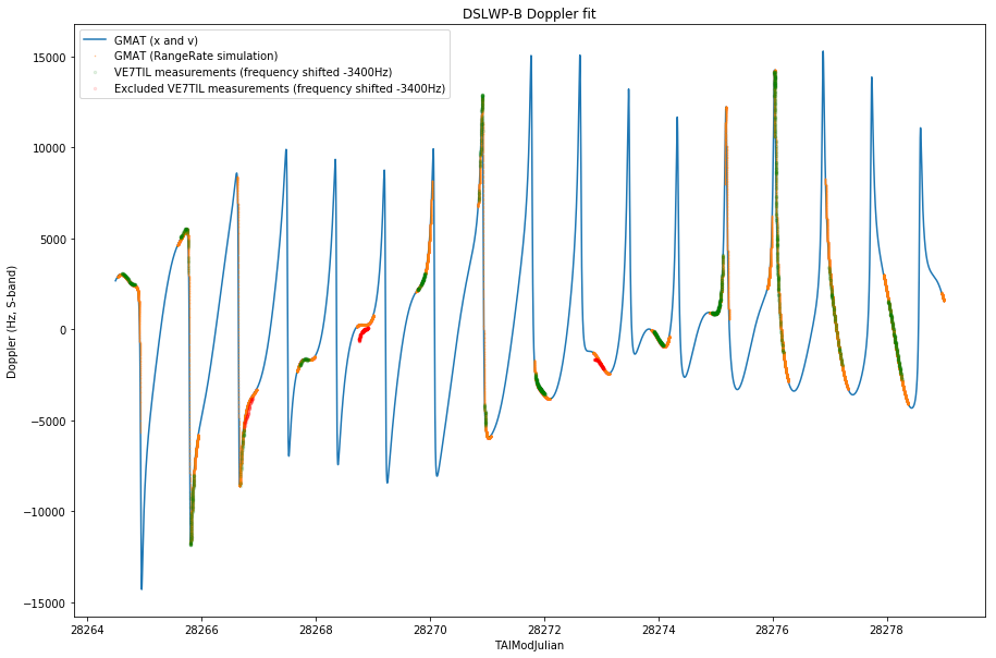
The Jupyter notebook where these calculations are performed can be found here.
1KUNS-PF image decoder
A week ago, Mike Rupprecht DK3WN told me that he had discovered JPEG images in the packets transmitted by 1KUNS-PF. I’ve had some time now to take a look at the information he sent me (including KISS dumps of the packets) and add an image decoder to gr-satellites.
JPEG images are not so difficult to spot amongst binary data, since they contain JFIF in ASCII in their header (4a 46 49 46 in hex). Another telltale sign of JPEG is the ff d8 ff that marks the start of the file. Presumably this is how Mike first noticed the images.
Mike has published some information about the image packets transmitted by 1KUNS-PF and he has been posting some of the images he receives.
Below there is the hex dump of the first and second packet CSP packet of a JPEG image (note the JFIF and ff d8 ff inside the packet payload).
pdu_length = 138
contents =
0000: 00 e2 92 42 00 00 ff d8 ff e0 00 10 4a 46 49 46
0010: 00 01 01 01 00 00 00 00 00 00 ff db 00 43 00 0c
0020: 08 09 0b 09 08 0c 0b 0a 0b 0e 0d 0c 0e 12 1e 14
0030: 12 11 11 12 25 1a 1c 16 1e 2c 26 2e 2d 2b 26 2a
0040: 29 30 36 45 3b 30 33 41 34 29 2a 3c 52 3d 41 47
0050: 4a 4d 4e 4d 2f 3a 55 5b 54 4b 5a 45 4c 4d 4a ff
0060: db 00 43 01 0d 0e 0e 12 10 12 23 14 14 23 4a 32
0070: 2a 32 4a 4a 4a 4a 4a 4a 4a 4a 4a 4a 4a 4a 4a 4a
0080: 4a 4a 4a 4a 4a 4a fa 14 dc 9e

pdu_length = 138
contents =
0000: 00 e2 92 42 00 01 4a 4a 4a 4a 4a 4a 4a 4a 4a 4a
0010: 4a 4a 4a 4a 4a 4a 4a 4a 4a 4a 4a 4a 4a 4a 4a 4a
0020: 4a 4a 4a 4a ff c4 00 1f 00 00 01 05 01 01 01 01
0030: 01 01 00 00 00 00 00 00 00 00 01 02 03 04 05 06
0040: 07 08 09 0a 0b ff c4 00 b5 10 00 02 01 03 03 02
0050: 04 03 05 05 04 04 00 00 01 7d 01 02 03 00 04 11
0060: 05 12 21 31 41 06 13 51 61 07 22 71 14 32 81 91
0070: a1 08 23 42 b1 c1 15 52 d1 f0 24 33 62 72 82 09
0080: 0a 16 17 18 19 1a 95 64 b7 7e
It seems that all the image packets are 138 bytes long. The first four bytes are the CSP header. Then we have 16bit big-endian field which counts the number of chunk, starting by 00. The last four bytes of the packet are most likely a checksum, and the remaining bytes are the corresponding chunk of the JPEG file.
I don’t know how to detect the end of one image other than by taking note of the beginning of the next image. In fact, this is the last packet of this image:
pdu_length = 138
contents =
0000: 00 e2 92 42 00 47 8a 00 5a 28 00 a2 81 05 14 00
0010: 51 40 05 14 00 51 40 05 14 00 51 40 05 14 00 51
0020: 40 c2 8a 00 28 a0 02 8a 00 28 a0 04 a2 80 0a 28
0030: 18 51 40 05 14 00 51 40 05 14 00 51 40 05 14 c6
0040: 14 50 01 45 00 14 50 01 45 00 14 50 01 45 00 14
0050: 50 01 45 00 14 50 01 45 00 7f ff d9 00 00 00 00
0060: 00 00 00 00 00 11 41 42 00 48 00 00 04 58 00 00
0070: 00 10 00 00 00 51 d0 38 c9 54 05 ac 8f d7 00 00
0080: bc 24 00 00 bc 24 dc bd 44 b0
The ff d9 that occurs mid-packet is the end-of-file of the JPEG file. I don’t know what to make of the rest of the data following it. Since not all of it is zero, it doesn’t look as deliberate padding. It might be the case that the satellite is sending information left over in a buffer.
The image below is the whole JPEG file contained in the packets received by Mike. It was sent using 72 chunks, for a total of 9216 bytes (at 128 bytes per chunk) and its resolution is 640×480. Most of the other images sent by 1KUNS-PF are smaller.

DSLWP-B’s journey to the Moon: part III
This is a follow-up on the series about DSLWP-B’s orbital dynamics (see part I and part II). In part I we looked at the tracking files published by Wei Mingchuan BG2BHC, which list the position and velocity of the satellite in ECEF coordinates, and presented basic orbit propagation with GMAT. In part II we explored GMAT’s capabilities to plan and perform manoeuvres, making a tentative simulation of DSLWP-B’s mid-course correction and lunar orbit injection. Now we turn to the study of DSLWP-B’s elliptical lunar orbit.
In this post we will examine the Keplerian elements of the orbits described by each of the tracking files published so far. We will also use Scott Tilley VE7TIL’s Doppler measurements of the S-band beacon of DSLWP-B to validate and determine the orbit.
DSLWP-B’s journey to the Moon: part II
This forms parts of a series of posts showing how to use GMAT to track the DSLWP-B Chinese lunar satellite. In part I we looked at how to examine and validate the tracking files published by BG2BHC using GMAT. It is an easy exercise to use GMAT to perform orbit propagation and produce new tracking files. However, note that the available tracking files come from orbit planning and simulation, not from actual measurements. It seems that the elliptical lunar orbit achieved by DSWLP-B is at least slightly different from the published data. We are already working on using Doppler measurements to perform orbit determination (stay tuned for more information).
Recall that there are three published tracking files that can be taken as a rough guideline of DSLWP-B’s actual trajectory. Each file covers 48 hours. The first file starts just after trans-lunar injection, and the second and third files already show the lunar orbit. Therefore, there is a gap in the story: how DSLWP-B reached the Moon.
There are at least two manoeuvres (or burns) needed to get from trans-lunar injection into lunar orbit. The first is a mid-course correction, whose goal is to correct slightly the path of the spacecraft to make it reach the desired point for lunar orbit injection, which is usually the lunar orbit periapsis (the periapsis is the lowest part of the elliptical orbit). The second is the lunar orbit injection, a braking manoeuvre to get the spacecraft into the desired lunar orbit and adjust the orbit apoapsis (the highest part of the orbit). Without a lunar orbit injection, the satellite simply swings by the Moon and doesn’t enter lunar orbit.
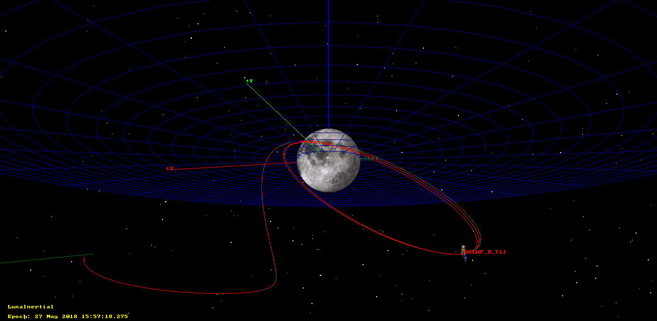
In this post we will see how to use GMAT to calculate and simulate these two burns, so as to obtain a full trajectory that is consistent with the published tracking files. The final trajectory can be seen in the figure below.