Experiments – Page 15 – Daniel Estévez

Frequency distribution of WSPR reports

Over the last few days I’ve been transmitting WSPR on 40m with 20dBm of power using my Hermes-Lite 2.0beta2. For this, I’m using the instrument output of the Hermes-Lite, which is driven by an OPA2677 200MHz dual opamp that produces a maximum output of 20dBm. I’ve been transmitting always on the frequency 7040100Hz. I have been collecting the reports from the WSPR database for a total of 2518 reports over 5 days of activity.

There are many statistics that can be done with this data, but since I have always been transmitting on the same frequency, it is quite interesting to look at the frequency in the reports. My Hermes-Lite is quite stable in frequency, as it uses a 0.5ppm 38.4MHz TCXO from Abracon. In fact, in the shack its stability is usually much better than 0.5ppm. During these tests I have verified the accuracy of the Hermes-Lite frequency by receiving my DF9NP 27MHz PLL, which is driven with a DF9NP 10MHz GPSDO. The 27MHz signal is usually reported around 3Hz high by the Hermes-Lite, with a drift of roughly 0.3Hz. This accounts for an error of 0.1ppm, and the drift is around 10ppb.

It seems that this performance is much better than the usual performance of the Amateur radio transceivers that report on the WSPR network, so the frequency reports can be used to measure the error of the frequency references in these Amateur radio transceivers. Noting that at 27MHz my Hermes-Lite is 3Hz low in frequency, I have determined a correction of -0.782Hz for my WSPR frequency, so I have chosen to take my transmission frequency as 7040099.218Hz when doing the calculations. This is probably accurate to a few tens of ppb.

I wanted to do a statistic of the distribution of the error in the frequency references of the WSPR receivers. To do this, I’ve decided that it’s better to first do, for each reporter, an average of the frequency of its reports, and then take this average as the frequency measured by that reporter. Then I do a histogram of the errors in the frequency reported by each reporter. The first average is done because there are some reporters which have a great number of reports with a very similar frequency (because their receiver might have an error, but it doesn’t drift much), and so the histogram would be biased with these reports if I just plotted the histogram of all the frequency reports. The histogram is shown below.

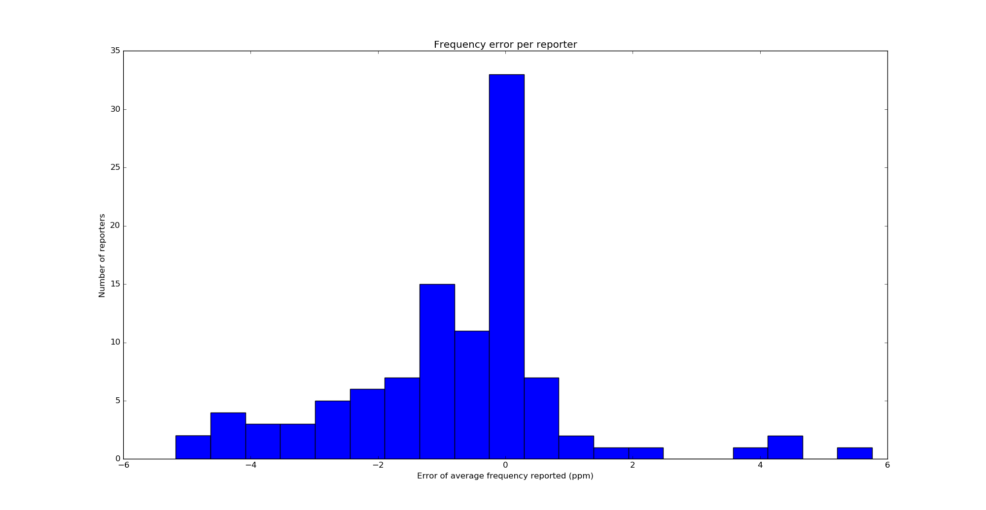
I find this histogram rather surprising. I expected to get a normal distribution or something similar, or at least a symmetric histogram centred on an error of 0ppm. However, the histogram is clearly skewed to the left. We conclude from this that a good number of WSPR receivers are quite accurate in frequency, and have an error of 0.5ppm or less. However, from those that are not accurate, it is much more probable that they are low in frequency (so they report me at a higher frequency).

I still have to find a good explanation for this effect. However, I have suspicions that this has something to do with the way that the frequency of a quartz crystal depends on the temperature (and this depends on the way that the crystal is cut). I have found in this document the image below.

Note that non-AT-cut crystals are low in frequency over most of the temperature range, so I can’t help but think that this is too much of a coincidence with the skew in my histogram above. Other people have pointed out that this is not so simple, as for instance the adjustment of the tuning capacitors of the crystal oscillator also plays an important role. It would be good to repeat this test in other bands and by other stations, perhaps in other parts of the world (my reporters come from Europe) and see if they also obtain a skewed histogram.

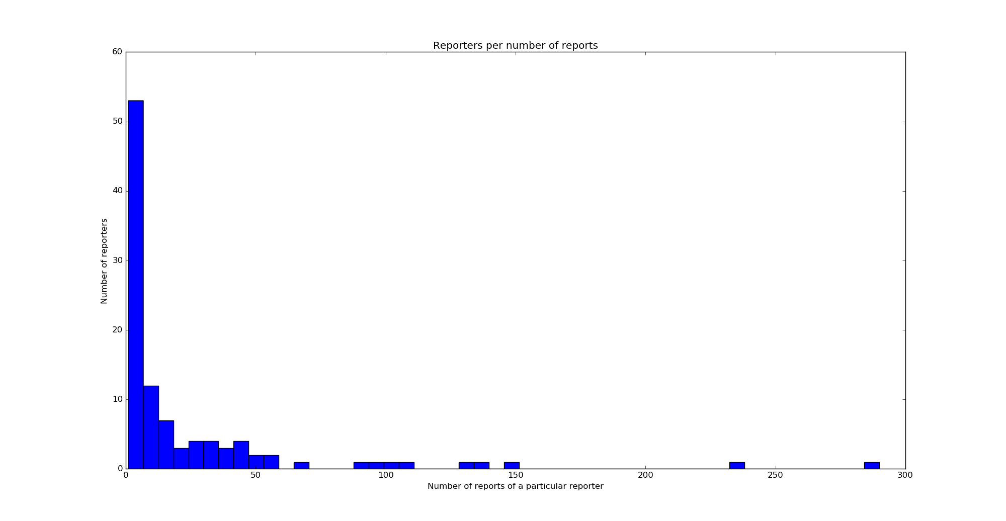
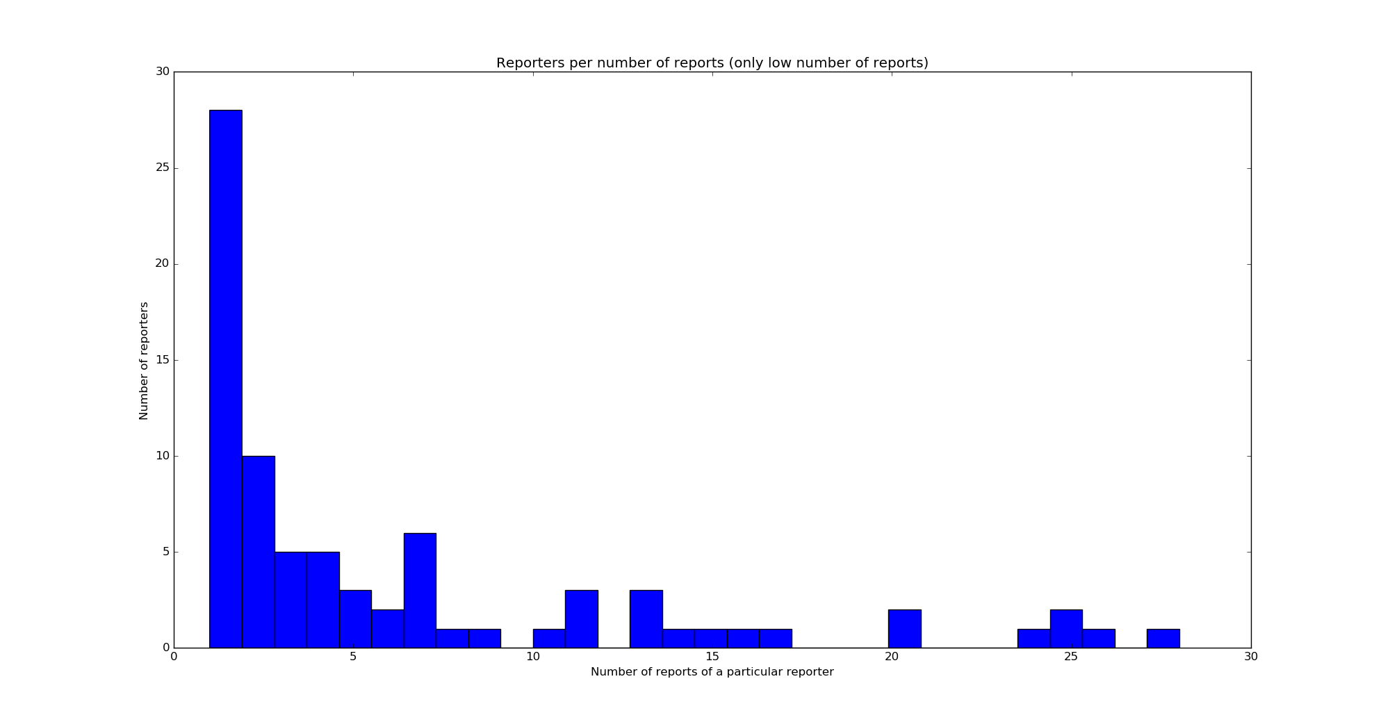
As an indication of the statistical significance of this test, I can say that a total of 2518 reports coming from 104 different reporters have been used. Just looking at these numbers is very far from doing a proper hypothesis contrast, but it is indicative that I have used a good amount of data. It is also interesting to look at the distribution of the number of reports given by each reporter. This is shown in the two histograms below (first for all numbers of reports and then for 30 reports and less).

The Python script and data used in this post are in this gist.

Acquisition and wipeoff for JT9A

Lately, I have been playing around with the concept of doing acquisition and wipeoff of JT9A signals, using a locally generated replica when the transmitted message is known. These are concepts and terminologies that come from GNSS signal processing, but they can applied to many other cases.

In GNSS, most of the systems transmit a known spreading sequence using BPSK. When the signal arrives to the receiver, the frequency offset (given by Doppler and clock error) and delay are unknown. The receiver runs a search correlating against a locally generated replica signal which uses the same spreading sequence. The correlation will peak for the correct values of frequency offset and delay. The receiver then mixes the incoming signal with the replica to remove the DSSS modulation, so that only the data bits that carry the navigation message remain. This process can be understood as a matched filter that removes a lot of noise bandwidth. The procedure is called code wipeoff.

The same ideas can be applied to almost any kind of signal. A JT9A signal is a 9-FSK signal, so when trying to do an FFT to visually detect the signal in a spectrum display, the energy of the signal spreads over several bins and we lose SNR. We can generate a replica JT9A signal carrying the same message and at the same temporal delay than the signal we want to detect. Then we mix the signal with the complex conjugate of the replica. The result is a CW tone at the difference of frequencies of both signals, which we call wiped signal. This is much easier to detect in an FFT, because all the energy is concentrated in a single bin. Here I look at the procedure in detail and show an application with real world signals. Recordings and a Python script are included.

WSJT-X and linear satellites: part I

Several weeks ago, in an AMSAT EA informal meeting, Eduardo EA3GHS wondered about the possibility of using WSJT-X modes through linear transponder satellites in low Earth orbit. Of course, computer Doppler correction is a must, but even under the best circumstances we cannot assume a perfect Doppler correction. First, there are errors in the Doppler computation because the TLEs used are always measured at an earlier time and do not reflect exactly the current state of the satellite. This was the aspect that Eduardo was studying. Second, there are also errors because the computer clock is not perfect. Even a 10ms error in the computer clock can produce a noticeable error in the Doppler computation. Also, usually there is a delay between the time that the RF signal reaches the antenna and the time that the Doppler correction is computed for and applied to the signal, especially if using SDR hardware, which can have large buffers for the signal. This delay can be measured and compensated in the Doppler calculation, but this is usually not done.

Here we look at errors of the second kind. We denote by \(D(t)\) the function describing the Doppler frequency, where \(t\) is the time when the signal arrives at the antenna. We assume that the correction is not done using \(D(t)\), but rather \(D(t – \delta)\), where \(\delta\) is a small constant. Thus, a residual Doppler \(D(t)-D(t-\delta)\) is still present in the received signal. We will study this residual Doppler and how tolerant to it are several WSJT-X modes, depending on the value of \(\delta\).

The dependence of Doppler on the age of the TLEs will be studied in a later post, but it is worthy to note that the largest error made by using old TLEs is in the along-track position of the satellite, and that this effect is well modelled by offsetting the Doppler curve in time. This justifies the study of the residual Doppler \(D(t)-D(t-\delta)\).

BER simulation in GNU Radio

David Rowe always insists that you should simulate the bit error rate for any modem you build. I’ve been intending to do some simulations of the decoders in gr-satellites since a while ago, and I’ve finally had some time to do so. I have simulated the performance of the LilacSat-1 decoder, both for uncoded BPSK and for the Viterbi decoder. This is just the beginning of the story, as the code can be adapted to simulate other modems. Here I describe some generalities about BER simulation in GNU Radio, the simulations I have done for LilacSat-1, and the results.

LilacSat-1 downlink usage

In my previous post, I examined a recording of LilacSat-1 transmitting an image. I did some calculations regarding the time it would take to transmit that image and the time that it actually took to transmit, given that the image was interleaved with telemetry packets. I wondered if the downlink KISS stream capacity was being used completely.

You can find more information about the downlink protocol of LilacSat-1 in this post. The important information to know here is that it consists of two interleaved channels: a channel that contains Codec2 frames for the FM/Codec2 repeater and a channel that contains a KISS stream. The KISS stream is sent at 3400bps. At any moment in time, the KISS stream can be either idling, by sending c0 bytes, or transmitting a CSP packet. The CSP packets can be camera packets (which are sent to CSP destination 6) or telemetry packets (and perhaps also other kinds of packets).

I have extracted the KISS stream from the recording and examined its usage to determine if it is being used at its full capacity or if it spends time idling. The image below represents the usage of each byte in the KISS stream, as time progresses. Bytes belonging to image packets are shown in blue, bytes belonging to other packets are shown in red and idle bytes are shown in white. (Remember that you can click the images to view them in full size).

The first 3 or 4 seconds of the graph are garbage, since the signal wasn’t strong enough. Then we see some telemetry packets and the image transmission starts. We observe that most image packets are transmitted leaving an idle gap between them. The size of the gap is similar to the size of the image packet. Every 10 seconds, a bunch of telemetry packets are transmitted, in a somewhat different order each time. Some telemetry packets are sent back to back, and others are interleaved with image packets. Image packets are only sent back to back just after a telemetry transmission.

The next graph shows the usage of the KISS stream averaged over periods of 5 secons. The y-axis means fraction of capacity of the link, so a 1 means that the full 3400bps are used. The capacity spent for image packets is shown in blue and the capacity used for telemetry is shown in red. The green curve is the sum of the blue and red, so it means the fraction of time that the link is not idle. We see that the link is never used completely. The total usage ranges between 60% and 90%, but never reaches 100%.

As expected, the capacity used for telemetry spikes up every 10 seconds. The blue curve is more interesting. It is roughly around 55%, but whenever telemetry is sent, it decreases a little. Just after each telemetry burst, the blue curve increases a little. This matches the behaviour we have seen in the previous graph. Every 10 seconds a telemetry burst is sent, using up some capacity that would normally be spent for image. After the telemetry burst, some image packets are sent back to back in a burst, peaking up to 60% capacity, but soon the packets continue being sent with idle gaps between them, and the capacity goes down to 55%.

It is a bit strange that the link is not fully utilised. One would expect that image packets are sent as fast as possible, stopping only to send telemetry. However, we have seen that there are many idle gaps. It seems that the image can’t be read very fast or that there is some other throttling mechanism. This would explain why a burst of image packets is sent after each telemetry burst: the image packets buffer up, because the link is sending telemetry. When the link is no longer busy with telemetry, it sends all the buffered image packets in a row, but soon enough image packets can’t be produced as fast as the link sends them, so idle gaps appear. This seems quite an important performance issue, as it appears that image transmission speed is capped at about 1870bps.

The Python code that generated these graphs can be seen below. The KISS file is also in the same gist.

Testing LilacSat-1 Codec2 downlink and GPS telemetry

Today I’ve finally had some time to test the LilacSat-1 Codec2 downlink on the air. I’ve been transmitting and listening to myself on the downlink during the 17:16 UTC pass over Europe from locator IN80do. The equipment used is a Yaesu FT-2D for the FM uplink, a FUNcube Dongle Pro+ and my decoder from gr-satellites for the downlink, and a handheld Arrow satellite yagi (3 elements on VHF and 7 elements on UHF). Here I describe the results of my test.

Waterfalls from QB50

In the previous post, I analysed a QB50 recording. Now I have prepared some waterfalls from my recording using the procedure I already described a while ago. The image above is obtained from a 1600×1024 waterfall with a resolution of 2.93kHz or 0.86s per pixel. I have labelled all the satellites and cropped it to a 1600×900 image that now I’m using as my desktop wallpaper.

I have also made a large 14120×16384 image with a resolution of 183.1Hz or 0.1s per pixel. The image can be downloaded here (142MB). I have found the following interesting crops within the large image. Remember that you can click on each image to view it in full size.

The fast fading that I detected in nSIGHT is clearly visible below. Note that the beacon period is almost, but not quite, an integer multiple of the fading period.

In the image below, we can see that SpaceCube is not very stable in frequency. The carrier frequency tends to rise rapidly each time that the transmitter goes on. Also, the overall trend is a frequency increase, counteracting the frequency decreasing effect of Doppler. This excerpt is near the end of SpaceCube’s pass, so the change in Doppler is not so large. The other French satellite, X-CubeSat, also shows a similar behaviour.

SpaceCube frequency instability

AAUSAT-4 usually transmits in 4k8 FSK using CCSDS FEC, but it also transmits a CW beacon sometimes. Both can be seen below.

AAUSAT-4 4k8 FSK and CW

Finally, a couple of CW satellites with interesting behaviour. On the upper part of the image below we can see BeEagleSat with fading. On the lower part, we can see Aalto-2 with its characteristic sidebands.

Fading in BeEagleSat and sidebands in Aalto-2

A tour of QB50

The QB50 project consists in a constellation of cubesats with the goal of studying the thermosphere. The cubesats are built by different universities around the world and each of them carries one of three different scientific instruments. A total of 36 cubesats have been built for the QB50 project. All of them transmit on the 70cm Amateur satellite band. A total of 28 were launched to the ISS on April 18th on the Cygnus CRS-7 resupply ship. Over the last two weeks, they have been released from the ISS. The complete launch schedule and radio information can be found here (note that the launches on May 23rd were delayed due to an unforeseen EVA). Several other non-QB50 cubesats, some of them transmitting in the Amateur bands, have also been released together with the QB50 satellites. This is probably the time that more Amateur satellite have been released at the same time. The satellites have not separated much yet, giving a great opportunity to record a single pass and analyse the telemetry of all the satellites.

A few days after the release of all the 28 QB50 cubesats, on May 29th at 18:25:29 UTC, I made an SDR recording of the complete pass of all the cubesats. The recording spans the 3MHz of the 70cm Amateur satellite band (435-438MHz) and lasts 23 minutes and 08 seconds. It was made from locator IN80do using a 7 element handheld yagi (the Arrow satellite yagi) held in the vertical polarization and a LimeSDR. The gain of the LimeSDR was set to maximum, but no external LNA was used. Here I look at the recording, list the satellites heard, and decode their telemetry.

Monitoring IMD levels in the EAPSK63 contest

This weekend I have recorded the full EAPSK63 Spanish PSK63 contest in the 40m band with the goal of playing back the recording later and reporting the stations showing excessively high IMD levels. In PSK contests, it is usual to see terribly distorted signals, which are the result of reckless operating techniques and stations which are setup inadequately. Contest rules don’t help much, as they are usually too weak to prevent distorted signals from interfering other participants. Amateurs should take care and strive to produce a signal as clean as possible. For instance, in the US, Part 97 101 a) states that “each amateur station must be operated in accordance with good engineering and good amateur practice”. Here I describe the signal processing done in this study and list a “hall of shame” of the worst stations I have spotted in my recording. I will notify by email the contest manager and all the stations in this list with the hope that the situation improves in the future.

First data from BY70-1

The Amateur satellite BY70-1 launched yesterday at around 3:00UTC. The launch was a partial failure, as all the satellites from this launch have been put in a 520x220km orbit. The perigee is too low to support a long duration orbit, and the satellites will decay in a couple months. BY70-1 has a 9k6 BPSK telemetry downlink on 70cm. This downlink is also used to download JPEG images from the onboard camera. I’ve talked about this in a previous post.

Since I’m at 33C3, I haven’t been able to receive this satellite with my own equipment yet. However, Tetsu JA0CAW already has posted some IQ recordings. Here I look at recording1 and recording2.

My first impression is that the packets are not very strong. I don’t know if this is something about JA0CAW’s station or that the downlink of BY70-1 is not very strong. I’ve only managed to decode the strongest packets in the recording. In comparison, LilacSat-2 has a very strong downlink and I can decode correctly almost from horizon to horizon with a handheld 7 element yagi.

Perhaps it’s possible to do some optimization of the decoder parameters such as filter width or loop bandwidths, but so far I haven’t experimented much. I just wanted to write a quick post to publish all the information I’ve managed to decode. I’m using the decoder from gr-satellites. The decoder log from recording1 is in this gist. From recording2 I could only decode a couple of JPEG packets and no telemetry packets.

There are three distinct types of telemetry packets. It seems that BY70-1 transmits all the three types in a single burst. Another curiosity: the message in one of the telemetry packets uses the callsign ON02CN, which is the Belgian callsign that LilacSat-1 will use. Since LilacSat-1 is part of the QB50 project, it makes sense that it uses a Belgian callsign. However, it seems that it’s some sort of software configuration error that BY70-1 is also using this callsign.

Update on 30/12/2016: I have found that there was a problem with the Costas loop bandwidth in the GNU Radio receiver on gr-satellites. Its value was too large. I have copied the value from the example demodulator on gr-lilacsat and now the decoder works much better. I have even been able to decode the following image from recording2.

The result looks pretty bad, but the keen eye will notice that in fact there are few packets lost in this JPEG image. Compare with the image posted by BG2BHC, which has no errors and is presumably the same image.