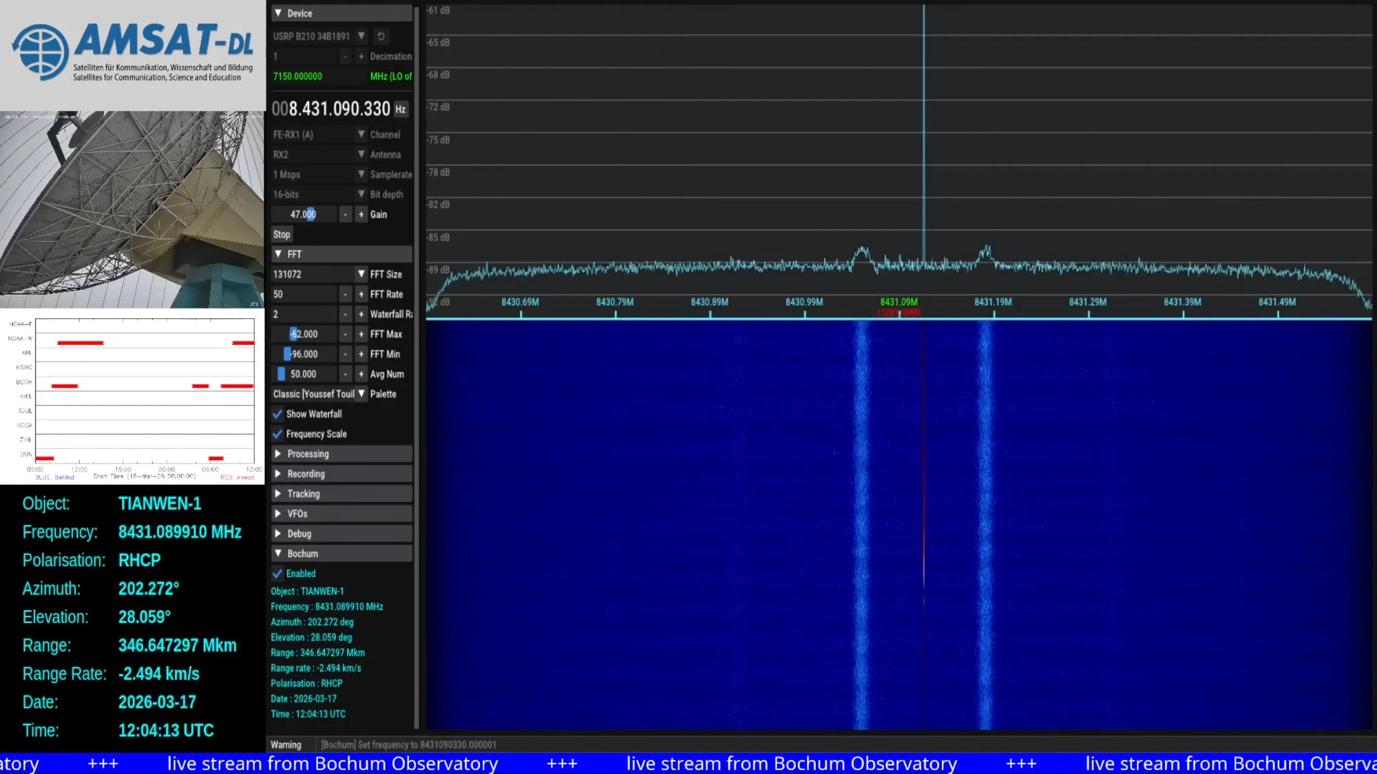
The signal strength looks completely normal, as evidenced by the spectrum plot shared in the announcement.
Screenshot of Tianwen-1 reception in Bochum shared by AMSAT-DL
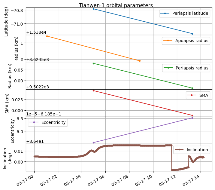
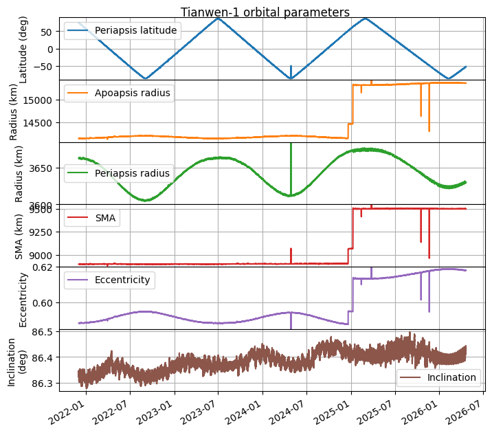
Telemetry containing state vectors was decoded between 2026-03-17 11:34 and 14:16 UTC. I have updated my plot of orbital parameters to include this new information. The period between 2025-12-23 and 2026-03-17 corresponds to a propagation with GMAT of the last telemetry received in 2025. The end of the plot corresponds to the telemetry received in 2026-03-17.
We can see that the orbit has remained the same, and there have been no manoeuvres during this period. A zoomed in version to the end of the plot shows that there is basically no jump in the orbital parameters. There is a tiny jump in the inclination as the new telemetry is received, but that is all.
So far the reasons why Tianwen-1 has apparently not transmitted telemetry to Earth for almost 3 months remain unknown.
Yesterday, AMSAT-DLpublished the news that they have been unable to receive any signals from Tianwen-1 with the 20 m antenna in Bochum since 2025-12-23. As you may know if you have been following my posts about Tianwen-1, AMSAT-DL has been using this antenna to receive and decode telemetry from Tianwen-1 almost every day since the beginning of the mission in 2020-07-23. The news about the lack of signal detected from Tianwen-1 over the last few months were hardly a secret, because AMSAT-DL runs a livestream of the signals received with the Bochum antenna 24/7, so anyone could look at the livestream and realize that Tianwen-1 was being observed but no signal was visible on the spectrum. However, now that the public has been made well aware of this fact, I can make some more comments about it. There has been no public communication from the Chinese space program regarding this, so the fate of Tianwen-1 is currently unknown.
During December 2025 and January 2026, there was a Mars conjunction, which means that Mars goes behind the Sun as seen from Earth. Communications with Mars orbiters cannot happen during this period of time. For instance, this news piece hints at NASA Mars missions not having contact between 2025-12-29 and 2026-01-16, which corresponds to a Sun-Earth-Mars angle (elongation) of 3º on 2025-12-29 and 1.8º on 2026-01-16, with the minimum elongation achieved on 2026-01-09. Therefore, it was completely expected that we would lose Tianwen-1’s signal during the conjunction period. Because the communications link to Earth does not work, spacecraft will usually not point their high gain antennas to Earth and even stop transmitting during this period. However, we expected to see Tianwen-1 back again after the conjunction, and we never did.
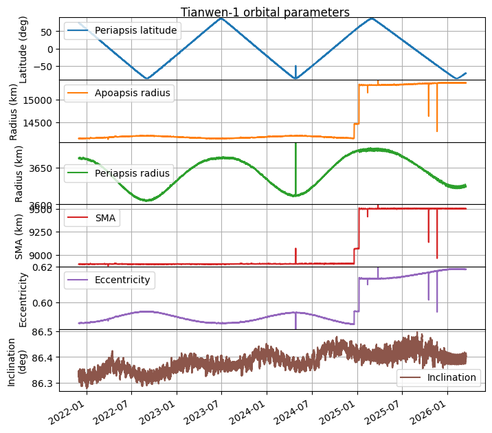
I have been using the telemetry decoded by AMSAT-DL, which includes the spacecraft state vectors, to keep track of the spacecraft orbit. I have been posting updates about any change that happens. The last one was the apoapsis raise on 2025-01-08. The lack of signals from Tianwen-1 sparked internal discussion about whether the spacecraft might have intentionally reentered some time around the conjunction period as a way of terminating the mission without leaving orbital debris. To analyse whether this could be possible, I have updated my orbit analysis to account for all the telemetry that has been received so far, up to 2025-12-22, which is when the last telemetry was decoded.
The result can be seen in the figure below. We see the apoapsis raises that happened during the end of 2024 and beginning of 2025. After that there have been no manoeuvres.
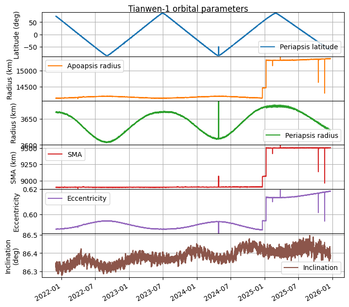
Since the plot above indicates that the periapsis radius would be going towards a minimum at the beginning of 2026 due to long-term periodic orbit perturbations, I propagated the last telemetry data we have forward with the goal of studying the impact of the larger apoapsis radius. The results are shown here. We note that the apoapsis radius minimum is now much higher than in the past, so the hypothesis of a reentry is unlikely unless a manoeuvre that we didn’t see in the telemetry has happened.
CSP is the Cubesat Space Protocol. It is a network protocol that was developed by Aalborg university, and is commonly used in cubesats, in particular those using GOMspace hardware. Initially the protocol allowed different nodes on a satellite to exchange packets over a CAN bus, but eventually it grew into a protocol that spans a network composed by nodes in the satellite and the groundstation that communicate over different physical layers, including RF links.
Recently I have been working on a project that involves CSP. To measure network performance and debug network issues, I have written some tooling in Rust, as well as a Wireshark dissector in Lua. The Rust tooling is an implementation from scratch and doesn’t use libcsp. Now I have open sourced these tools in a csp-tools repository and csp-tools Rust crate. In this post I showcase how the tools work.
In my previous post I decoded a transmission from a V16 beacon. The V16 beacon has mandatorily replaced warning triangles in Spain in 2026. It is a device that contains a strobe light and an NB-IoT modem that sends its GNSS geolocation using the cellular network. It is said that the beacon first transmits is geolocation 100 seconds after it has been powered on, and then it transmits it again every 100 seconds. In that post I recorded one of those transmissions done after the beacon had been powered on for a few minutes and I decoded it by hand. I showed that the transmission contains a control plane service request NAS message that embeds a 158 byte encrypted message, which is what presumably contains the geolocation and other beacon data.
In that post I couldn’t show how the beacon connects to the cellular network and sets up the EPS security context used to encrypt the message, since that would have happened some minutes before I made the recording. I have now made a recording that contains both the NB-IoT uplink and the corresponding NB-IoT downlink and starts before the V16 beacon is switched on. In this post I show the contents of the uplink recording.
The V16 beacon is a car warning beacon that will mandatorily replace the warning triangles in Spain starting in 2026. In the event of an emergency, this beacon can be magnetically attached to the roof of the car and switched on. It has a bright LED strobe light and a connection to the cellular network, which it uses to send its GNSS position to the DGT 3.0 cloud network (for readers outside of Spain, the Spanish DGT is roughly the equivalent of the US DMV). The main point of these beacons is that placing warning triangles far enough from a vehicle can be dangerous, while this beacon can be placed without leaving the car.
There has been some criticism surrounding the V16 beacons and their mandatory usage that will start in January 2026, both for economical and implantation roadmap reasons, and also for purely technical reasons. The strobe light is so bright that you shouldn’t look at it directly while standing next to the beacon (which makes it tricky to pick it up and switch it off), but I have heard that it is not so easy to see in daylight from several hundreds of meters away.
The GNSS geolocation and cellular network service is also somewhat questionable. I purchased a V16 beacon from the brand NK connected (certificate number LCOE 2024070678G1), for no reason other than the fact that it was sold in a common supermarket chain. The instructions in the box directed me to the website validatuv16.com for testing it. In this website you can register the serial number or IMEI of your beacon and your email. Then you switch on the beacon. After 100 seconds the beacon should send a message to the DGT network, and then periodically every 100 seconds. This test service is somehow subscribed to the DGT network, and it sends you an email that contains the message data (GNSS position and battery status) when the DGT network receives it. This is great, but there is no test mode or anything that declares that you are using the beacon just for testing purposes. They only say that you should not leave the beacon on for much longer than what it takes you to receive the email, to avoid the test being mistaken for a real emergency. The fact that the test procedure for this system is literally the same as the emergency procedure is a red flag for me. Additionally, this beacon only includes cellular data service for 12 years, and it is not clear what happens after that.
Technical shortcomings aside, my main interest is how the RF connection to the DGT network works. The beacon I bought has a logo in the box saying that it uses the Orange cellular network. When I tested it, after receiving the confirmation email from the test service, I used a Pluto SDR running Maia SDR and quickly found that the beacon was transmitting NB-IoT on 832.3 MHz. I made a recording of one of the periodic transmissions. In this post I analyse and decode the recording.
A few days ago I was doing some refactoring of my galileo-osnma project. This is a Rust library that implements the Galileo OSNMA (open service navigation message authentication) system. The library includes a demo that runs in a Longan nano GD32VF103 RISC-V microcontroller board. The purpose of this demo is to show that this library can run on small microcontrollers. My refactoring was in principle a simple thing: I was mainly organizing the repository as a Cargo workspace, and unifying the library and some supporting tools into the same crate. However, after the refactor, users reported that the Longan nano software was broken. It would hang after processing some messages. This post is a collection of notes about how I investigated the issue, which turned out to be related to stack usage.
I have published a new Python package called sigmf-toolkit. It is intended to be a collection of Python tools to work with SigMF files. At the moment it only contains two tools, but I plan on adding more tools to this package as the needs arise. These tools are:
gr_meta_to_sigmf. It converts a GNU Radio metadata file with detached headers to a SigMF file. At the moment it is really simple, and it doesn’t handle capture discontinuities.
sigmf_pcap_annotate. This tool parses a PCAP file using Scapy and it adds annotations to a SigMF file for each packet in the PCAP file.
I find this sigmf_pcap_annotate tool quite useful when comparing side by side a SigMF file in Inspectrum and a PCAP file in Wireshark to debug issues with digital communications systems. In this post I showcase how this tool can be used.
Today marks 10 years since I wrote the first post in this blog. It was a very basic and brief post about me decoding the European FreeDV net over a WebSDR. I mainly wrote it as a way of getting the ball rolling when I decided to start a blog back in October 2015. Over the 10 years that I have been blogging, the style, topics, length and depth of the posts have kept shifting gradually. This is no surprise, because the contents of this blog are a reflection of my interests and the work I am doing that I can share freely (usually open source work).
Since I started the blog, I have tried to publish at least one post every month, and I have managed. Sometimes I have forced myself to write something just to be up to the mark, but more often than not the posts have been something I really wanted to write down and release to the world regardless of a monthly tally. I plan to continue blogging in the same way, and no doubt that the contents will keep evolving over time, as we all evolve as persons during our lifetime. Who knows what the future will bring.
I wanted to celebrate this occasion by making a summary of the highlights throughout these 10 years. I have written 534 posts, and although Google search is often useful at finding things, for new readers that arrive to this blog it might be difficult to get a good idea of what kind of content can be found here. This summary will be useful to expose old content that can be of interest, as well as serve me to reflect on what I have been writing about.
In February this year I was in the Spanish amateur microwave radio conference Micromeet 2025. In this conference, Luis Cupido CT1DMK presented a simple and inexpensive 10 GHz transverter that he called Nes-Transverter, with the motto “Instant microwaves. Just add solder”. The main idea of this design is that it is very simple and can be built by anyone with just a handful of inexpensive components. Luis was hoping that this project would help more people get on the 10 GHz band in a hands-on way, and he also wanted to demystify some ideas such as amateur microwave radio being difficult or expensive.
The schematic for this design is available here. It uses a 144 MHz IF, allowing it to be connected to a VHF amateur radio. An ADF4351 synthesizer, to be sourced from an inexpensive AliExpress dev board, generates a 2.556 GHz LO with complementary outputs. These two outputs are used in a frequency doubler built with two BAT15 diodes to produce a 5.112 GHz LO, which is filtered with a transmission line stub and amplified with an MMIC such as the ERA 3+. A harmonic x2 mixer built with two BAT15 diodes directly connected to the waveguide probe uses the 5.112 GHZ LO and the 144 MHz IF to produce 10.368 GHz, which is the usual frequency for terrestrial narrowband communications in the 10 GHz amateur band.
I was very interested by this talk, and thought that it would be fun to play with this project, since I haven’t done any hands-on electronics projects in quite a while. However, rather that building a transverter for narrowband communications, I decided to adapt the ideas to build a 10 GHz FMCW radar. I wanted to build a cheaper version of the ADALM-PHASER, minus the phased array part. The Phaser is an educational development kit from ADI that demonstrates concepts in phased array beamforming and FMCW radar. It uses an ADF4159 waveform generator synthesizer and a HMC735 VCO as a 12.2-12.7 GHz LO source that can be programmed to generate FMCW waveforms such as a linear sawtooth and triangle chirps. An ADALM-PLUTO or another SDR is used as a 2.2 GHz IF to obtain 10-10.5 GHz via high-side LO injection. On the transmit section, the 10-10.5 GHz signal is sent to an SMA connector to drive an external antenna. On the receive section, a 4×8 phased array of patches is included in the PCB. Each column of 4 patches is phased as a single element by connecting them together on the PCB. The 8 columns are beamformed in groups of 4 with two ADAR1000, which allows choosing independent complex coefficients for each column. Each of the 4-column beamformer outputs is connected to an RX channel of a 2-channel SDR, so that the final beamforming step can happen in software (see here for a block diagram of the Phaser).
The first thing I needed to replace in Luis design to convert it to an FMCW radar was the LO source. Since I will be using an SDR rather than a VHF radio as the IF, I could use an LO of around 4-4.5 GHz, which would give me around 10-10.5 GHz with an IF around 1-2 GHz. This meant that I could use the ADF4158 synthesizer as the LO source. This is the cheaper variant of the ADF4159, and it only goes up to 6.1 GHz instead of 13 GHz, which is fine for my use case. I needed a VCO to go together with the synthesizer, and after some looking around I decided to use another ADI part, the HMC319, which is a 3.9-4.45 GHz VCO. An IF of 1.6 GHz covers 10-10.5 GHz with an LO of 4.2-4.45 GHz, which is quite appropriate for this VCO choice.
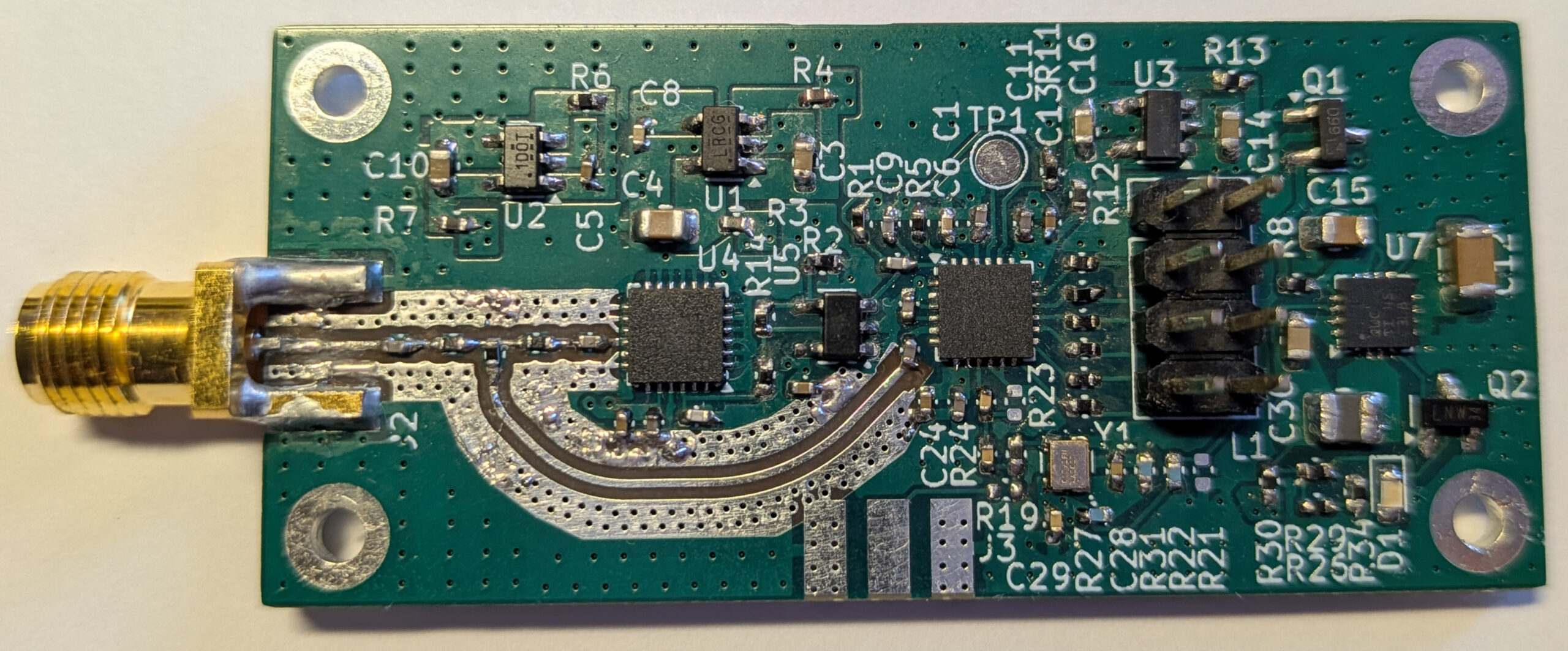
I designed a small PCB with an ADF4158 and HMC391, which I now have built and tested. In this post I explain some of the aspects of the board design and the results of the initial tests.
In my last post about 5G NR, which was part of a series in which I analyzed the signals in a short recording of an idle srsRAN gNB, I mentioned that I had already decoded all the signals that appear in the recording, and that to move on with my 5G series I would need to make and use some more complex real world recordings next.
A 5G band I’m particularly interested in is n78 (3.3 – 3.8 GHz TDD). This is being used to deploy 5G in many European countries, including Spain, as showed by this list in Wikipedia. Due to the large bandwidth available, it is common to see cells with 100 MHz bandwidth in this band.