Satellite RF signals are shifted in frequency proportionally to the line-of-sight velocity between the satellite and groundstation, due to the Doppler effect. The Doppler frequency depends on time, on the location of the groundstation, and on the orbit of the satellite, as well as on the carrier frequency. In satellite communications, it is common to correct for the Doppler present in the downlink signals before processing them. It is also common to correct for the uplink Doppler before transmitting an uplink signal, so that the satellite receiver sees a constant frequency.
For Earth satellites, these kinds of corrections can be done in GNU Radio using the gr-gpredict-doppler out-of-tree module and Gpredict (see this old post). In this method, Gpredict calculates the current Doppler frequency and sends it to gr-gpredict-doppler, which updates a variable in the GNU Radio flowgraph that controls the Doppler correction (for instance by changing the frequency of a Frequency Xlating FIR Filter or Signal Source).
I’m more interested in non Earth orbiting satellites, for which Gpredict, which uses TLEs, doesn’t work. I want to perform Doppler correction using data from NASA HORIZONS or computed with GMAT. To do this, I have added a new Doppler Correction C++ block to gr-satellites. This block reads a text file that lists Doppler frequency versus time, and uses that to perform the Doppler correction. In this post, I describe how the block works.
The Doppler Correction block is shown below.
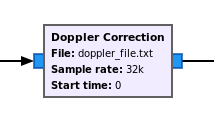
The text file that it uses as input lists one timestamp and Doppler frequency per line. The timestamp is given in seconds, typically using the UNIX epoch, and the Doppler frequency is given in Hz. The timestamp and frequency are separated by a space. An example of a few lines of a Doppler file is shown here:
1657342799.9999733 6347.772154386505
1657342814.4000158 6336.4809640557505
1657342828.800018 6325.186964971246
The block keeps track of time internally by using the sample rate and the timestamp corresponding to the first sample that it processes. This can be specified using the “Start time” parameter of the block, which is useful when processing recordings. When using the “Start time” parameter, the time scale of the start time in the block and the timestamps in the file need to match, but it is not mandatory to use UNIX time.
The block also understands rx_time stream tags, such as those generated by UHD. If the block sees an rx_time tag in its input, it will update its internal time as indicated by the tag. In this case it is necessary to use UNIX timestamps in the Doppler file, since rx_time tags use UNIX time. This allows us to use the UHD Source block with a USRP whose time has been set previously. In this case, the “Start time” parameter can be set to 0, as the UHD Source block will send and rx_time tag with its first sample.
For each input sample, the block determines its associated timestamp \(t\), computes the Doppler frequency \(f(t)\) by linearly interpolating between the two neighbouring values given in the file, and then applies a continuous-phase frequency shift of \(-f(t)\) to the input signal to produce the output. This gives a really precise Doppler correction if the lines in the file use small steps (the appropriate step size should be determined in terms of the curvature of the Doppler vs. time function).
For timestamps before the first entry of the file or after the last entry, the frequency value of the first or last entry is used (i.e., the frequency is held constant outside of the time range described by the file).
The text file describing the Doppler curve can be generated easily. The example code below shows how to use Astroquery to fetch data from NASA HORIZONS and format it appropriately. The example corresponds to an observation of Voyager-1 from the Allen Telescope Array. Since the Doppler frequency is quite large (on the order of -820 kHz), most of the Doppler is handled by tuning the receiver 820 kHz below the transmit frequency, so the Doppler file actually contains the difference between the Doppler and -820 kHz.
from astroquery.jplhorizons import Horizons
from scipy.constants import c
from astropy.time import Time

spacecraft_freq = 8420.432097e6

observatory_code = -72 # set to -72 for HCRO, -9 for GBT
query = Horizons(
    id = 'Voyager 1', location=str(observatory_code),
    epochs = {'start': '2022-07-09 05:00:00',
              'stop': '2022-07-09 09:00:00',
              'step': '1000'},
    )
eph = query.ephemerides()
doppler = -eph['delta_rate']*1e3/c*spacecraft_freq

average_doppler = -820e3
baseband_freq = doppler - average_doppler

ts = Time(eph['datetime_jd'], format='jd').unix
fs = baseband_freq.value.data
with open('/tmp/voyager1_doppler.txt', 'w') as doppler_file:
    for t, f in zip(ts, fs):
        print(t, f, file=doppler_file)
I wanted to have a Doppler correction block like this since quite a while, but I finally implemented it just a couple of weeks ago, while I was visiting the Allen Telescope Array. We wanted to observe Voyager-1, and I figured out that this block would be quite useful to correct the Doppler in real time and let us see the signal in the integrated spectrum. The example code above is in fact the one I used for the ATA observation.
I validated this block by using the Voyager-1 recording that I did with the ATA back in November 2020. Originally, I made a Jupyter notebook where the Doppler correction was done in Python with Dask. I ran the recording through the Doppler correction block, removed the Doppler correction from the Python code, and obtained very similar results to the original ones.
We also tested the block by observing Voyager-1 with two ATA antennas and the two USRP N32x in the GR-ATA Testbed, correcting the Doppler in real time, and recording Doppler corrected IQ data to disk. We also recorded data with the ATA 20-antenna beamformer during the same observation. Later, I ran this recording through the Doppler correction block. All these tests showed good results, with the Doppler corrected signal occupying a bandwidth of around 0.5 to 1 Hz.
After using this block successfully at the ATA, I had it lying around in an ad-hoc out-of-tree module that I hadn’t published yet. Rather than publishing the code as such and perhaps letting it bit rot, I have decided to add the block to gr-satellites so that it’s easier for me to maintain. The block isn’t currently used anywhere in gr-satellites, but maybe some gr-satellites users will find it useful.
A simple example of the Doppler Correction block is included in gr-satellites. A text file describes a Doppler curve that first follows a sinusoid and then grows linearly. The input to the Doppler Correction block is the constant 1, so at the output we get a CW carrier of the opposite frequency to the one given in the Doppler file.
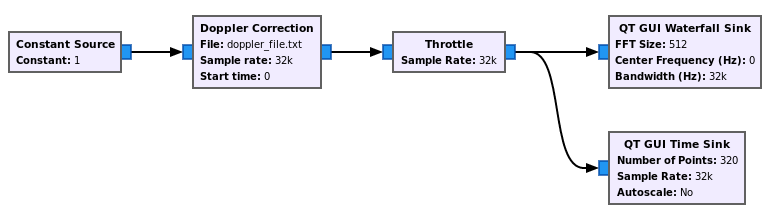
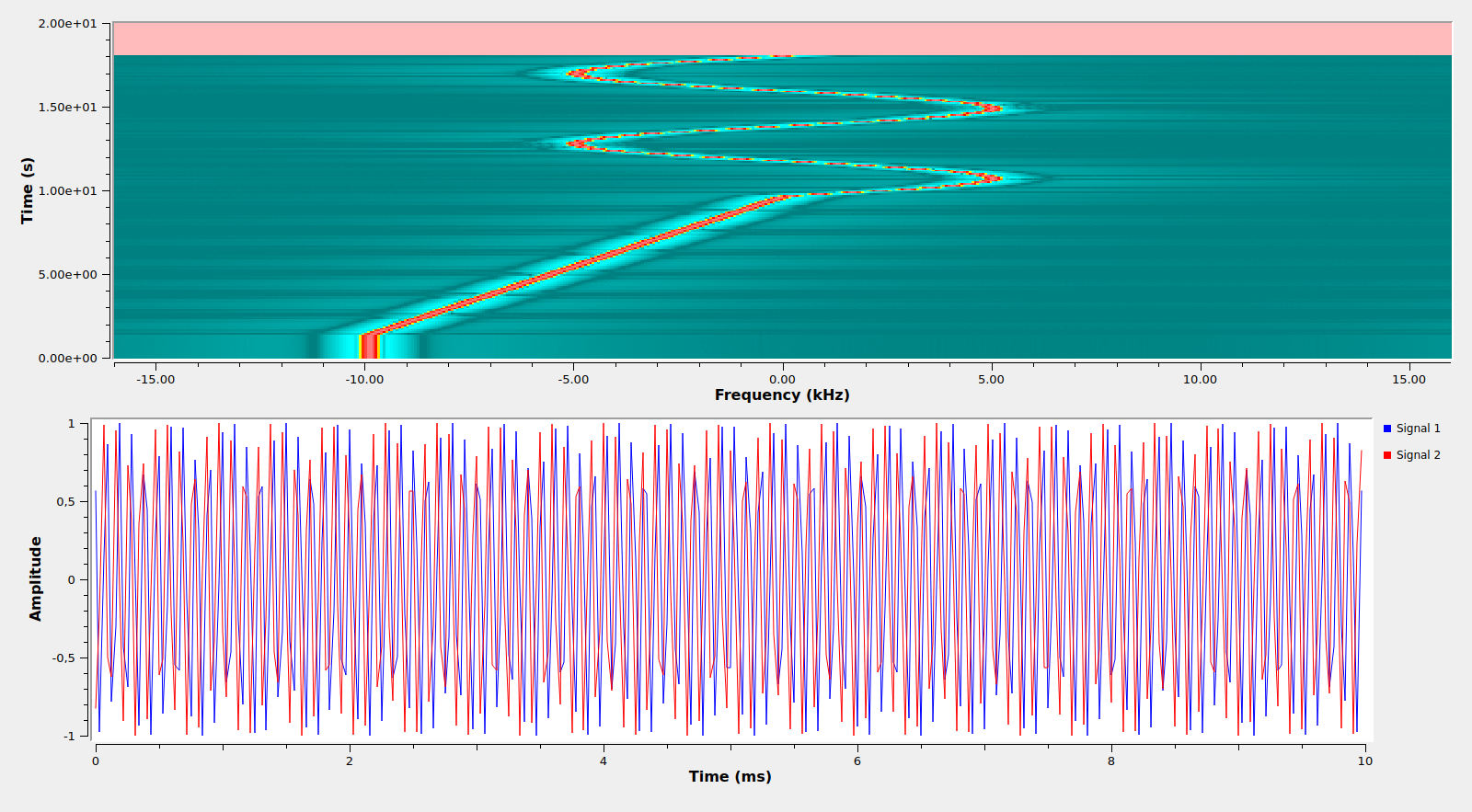
The figure below shows the GUI output of the example after the time interval described in the Doppler file has finished. We can see the sinusoid and linear slope in the waterfall.
If we write the output of the Doppler Correction block to a file, we can see the Doppler curve more clearly by using Inspectrum.

Thank you for adding that to gr-satellites for general availability! One difficulty w/ replaying an I/Q file in GNU Radio is that the signal of interest is often not centered in the passband and commonly will experience doppler frequency changes throughout the duration of the recording.
Could this block be used to ‘track’ a signal from a known object to allow for demodulation throughout all or most of the recording? If so, how would someone generate the required text file for objects not in Horizons but rather from a conventional TLE.
Thanks!
Yes, this can be done. For instance the Python library Skyfield can be used to compute Dopplers from a TLE. See for example cells [3] through [6] in this notebook. After this has been done, we will have the UNIX timestamps and Doppler frequencies in Numpy vectors and we can write the Doppler text file as in the HORIZONS example above.
Hi Daniel. First I want to thank you for making so much material available at the GNURADIO level. It has helped me a lot in learning.
I would like to know if there is any tutorial that teaches using the Doppler Correction block to correct the Doppler of a nanosatellite with an orbit similar to that of the ISS, using Gpredict or orbitron. Thank you very much in advance.
Hi, this Doppler correction block is intended to be used with a text file prepared beforehand. You could prepare the text file starting from a TLE with some Python code. But it doesn’t interface with Gpredict. If you want to get Doppler correction data from Gpredict into GNU Radio, then you can use gr-gpredict-doppler.
And do you know any Python code that converts the TLE in this file?
We’ll need it for two weeks from now, and we won’t have time to develop.
Thank you very much in advance.
Maybe Skyfield is useful for this.
Hi Daniel,
I hope you are doing well. I don’t fully understand the usage of the “Start Time” parameter in this block. Would you mind describing further how this block works? I ultimately want to pass the time at which the gnuradio software is started as the “Start Time.” Here is some info on what we tried and observed:
We generated a file with pairs of UNIX timestamps and doppler shifting frequencies as davised. The time stamps in this file corresponds to when our satellite is passing over head. In the “Start Time” parameter, we have tried passing time.time() and an actual float of the current UNIX time, but the resulting signal appears to only be using the first line of the requested doppler correction from the file. We also observed gnuradio’s debug print state that the doppler_correction block sets time ~0 at sample 0, so we assume the doppler correction block must be setting start time as the beginning of the UNIX epoch instead of at the “current” time we passed in the “Start Time” parameter.
When we edited the file and shifted all the timestamps back so the first timestamp is 0 seconds, the doppler correction block works as expected.
Is this consistent with what you are expecting and we are using the block incorrectly? How should we pass the “current” (whenever the program is initiated) timestamp to the “Start Time” parameter?
Thank you so much for all your work on gr-satellites! It has been very useful for our lab’s satellite operations.
The “Start time” parameter is in units of seconds and must match the scale you use in your .txt file. Normally you would use UNIX timestamps for both. However, the “Start time” parameter is overridden if the block receives an rx_time tag from a UHD Source block (or a pck_n tag from a gr-difi source block). I think this is what is happening in your case. You have a USRP in your setup which is sending and rx_time of zero in the first sample (that’s why you get such debug message). You should either set the USRP clock to UNIX time using the UHD API (preferred solution) or block the tags using a Tag Gate block.
Thank you for your reply. That makes sense. As a work around, I added another rx_time tag with the current UNIX time on sample 1 (after the USRP’s rx_time tag on sample 0). We’ll use this for now while we work on syncing the USRP clock to UNIX time.
Hello, I want to simulate Doppler shift, with GNU and USRP-B200, and inject frequency with RF generator for deep space mission but after simulate with blocks , only I can see waterfall and peak frequency, and I don’t know how do I have fix it. I used for Rx: USRP Source+LPF+File sink and QT GUI frequency sink and QT GUI Waterfall Sink , and for Tx : File source +90 sec delay+multiply0 with siganl source +multiply const+VCO(complex) +multiply1 then output of multiply goes to USRP Sink+ QT GUI frequncy sink, after turn on RF generator, I can see Peak RF at -45 dB, as I injected RF gen -30 dB and waterfall shows moving
Hi Keivan, I cannot provide support for this over comments in the blog, specially since your question is only tangentially related to the GNU Radio block introduced in this post.