Even though the cubesat LilacSat-1 was launched more than a year ago, I haven’t played with it much, since I’ve been busy with many other things. I tested it briefly after it was launched, using its Codec2 downlink, but I hadn’t done anything else since then.
LilacSat-1 has an FM/Codec2 transponder (uplink is analog FM in the 2m band and downlink is Codec2 digital voice in the 70cm band) and a camera that can be remotely commanded to take and downlink JPEG images (see the instructions here). Thus, it offers very interesting possibilities.
Since I have some free time this weekend, I had planned on playing again with LilacSat-1 by using the Codec2 transponder. Wei Mingchuan BG2BHCpersuaded me to try the camera as well, so I teamed up with Mike Rupprecht DK3WN to try the camera this morning. Mike would command the camera, since he has a fixed station with more power, and we would collaborate to receive the image. This is important because a single bit error or lost chunk in a JPEG file ruins the image from the point where it happens, and LilacSat-1 doesn’t have much protection against these problems. By joining the data received by multiple stations, the chances of receiving the complete image correctly are higher.
A couple months ago, Andrés Calleja EB4FJV installed a 2.3GHz beacon in his home in Colmenar Viejo, Madrid. The beacon has 2W of power, radiates with an omnidirectional antenna in the vertical polarization, and transmits a tone and CW identification at the frequency 2320.865MHz.
Since Colmenar Viejo is only 10km away from Tres Cantos, where I live, I can receive the beacon with a very strong signal from home. The Madrid-Barajas airport is also quite near (15km to the threshold of runway 18R) and several departure and approach aircraft routes pass nearby, particularly those flying over the Colmenar VOR. Therefore, it is quite easy to see reflections off aircraft when listening to the beacon.
On July 8 I did a recording of the beacon from 10:04 to 11:03 UTC from the countryside just outside Tres Cantos. In this post I will examine the aircraft reflections seen in the recording and match them with ADS-B aircraft position and velocity data obtained from adsbexchange.com. This will show the locations and trajectories which produce reflections strong enough to be detected.
In one of my latest posts I analysed the meteor scatter pings from GRAVES on a recording I did on August 11 (see that post for more details about the recording). The recording covered the frequency range from 142.5MHz to 146.5MHz and was 1 hour and 34 minutes long. Here I look at the Amateur stations that can be heard in the recording. Note that Amateur activity in meteor scatter communications increases considerably during large meteor showers, due to the higher probabilities of making contacts.
I have a DF9NP 10MHz GPSDO that is based on a u-blox LEA-5S GPS receiver. Essentially, the LEA-5S outputs an 800Hz signal that is used to discipline a 10MHz VCTCXO with a PLL. The LEA-5S doesn’t have persistent storage, so an I2C EEPROM is use to store the settings across reboots.
Lately it seemed that the reading of the settings from the EEPROM had failed. The u-blox was always booting with the default settings. This prevents the GPSDO from working, since the default for the timepulse signal is 1Hz instead of 800Hz. Here is the summary of my troubleshooting session and the weird repair that I did.
The SiriusSats are using 4k8 FSK AX.25 packet radio at 435.570MHz and 435.670MHz respectively, using callsigns RS13S and RS14S. The Tanushas transmit at 437.050MHz. Tanusha-3 normally transmits 1k2 AFSK AX.25 packet radio using the callsign RS8S, but Mike Rupprecht sent me the other day a recording of a transmission from Tanusha-3 that he could not decode.
It turns out that the packet in this recording uses a very peculiar modulation. The modulation is FM, but the data is carried in audio frequency phase modulation with a deviation of approximately 1 radian. The baudrate is 1200baud and the frequency for the phase modulation carrier is 2400Hz. The coding is AX.25 packet radio.
Why this peculiar mode is used in addition to the standard 1k2 packet radio is a mystery. Mike believes that the satellite is somehow faulty, since the pre-recorded audio messages that it transmits are also garbled (see this recording). If this is the case, it would be very interesting to know which particular failure can turn an AFSK transmitter into a phase modulation transmitter.
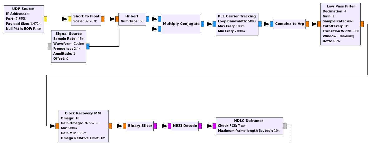
I have added support to gr-satellites for decoding the Tanusha-3 phase modulation telemetry. To decode the standard 1k2 AFSK telemetry direwolf can be used. The decoder flowgraph can be seen in the figure below.
TANUSHA-3 gr-satellites decoder
The FM demodulated signal comes in from the UDP source. It is first converted down to baseband and then a PLL is used to recover the carrier. The Complex to Arg block recovers the phase, yielding an NRZ signal. This signal is lowpass filtered, and then clock recovery, bit slicing and AX.25 deframing is done. Note that it is also possible to decode this kind of signal differentially, without doing carrier recovery, since the NRZI encoding used by AX.25 is differential. However, the carrier recovery works really well, because there is a lot of residual carrier and this is an audio frequency carrier, so it should be very stable in frequency.
The recording that Mike sent me is in tanusha3_pm.wav. It contains a single AX.25 packet that when analyzed in direwolf yields the following.
RS8S>ALL:This is SWSU satellite TANUSHA-3 from Russia, Kursk<0x0d>
------
U frame UI: p/f=0, No layer 3 protocol implemented., length = 68
 dest    ALL     0 c/r=1 res=3 last=0
 source  RS8S    0 c/r=0 res=3 last=1
  000:  82 98 98 40 40 40 e0 a4 a6 70 a6 40 40 61 03 f0  ...@@@...p.@@a..
  010:  54 68 69 73 20 69 73 20 53 57 53 55 20 73 61 74  This is SWSU sat
  020:  65 6c 6c 69 74 65 20 54 41 4e 55 53 48 41 2d 33  ellite TANUSHA-3
  030:  20 66 72 6f 6d 20 52 75 73 73 69 61 2c 20 4b 75   from Russia, Ku
  040:  72 73 6b 0d                                      rsk.
------
The contents of the packet are a message in ASCII. The message is of the same kind as those transmitted in AFSK.
GRAVES is a French space surveillance radar that transmits with very high power at 143.050MHz. It is easy to receive it from neighbouring countries via meteor scatter. During this year’s Perseids meteor shower I did a recording of GRAVES and the 2m Amateur band for later analysis. The recording was done at 08:56 UTC of Saturday 12th August and it is about 1 hour and 34 minutes long. Here I present an algorithm to detect and extract the meteor scatter pings from GRAVES.
If you’ve being following my latestposts, probably you’ve seen that I’m taking great care to decode as much as possible from the SSDV transmissions by DSLWP-B using the recordings made at the Dwingeloo radiotelescope. Since Dwingeloo sees a very high SNR, the reception should be error free, even without any bit error before Turbo decoding.
However, there are some occasional glitches that corrupt a packet, thus losing an SSDV frame. Some of these glitches have been attributed to a frequency jump in the DSLWP-B transmitter. This jump has to do with the onboard TCXO, which compensates frequency digitally, in discrete steps. When the frequency jump happens, the decoder’s PLL loses lock and this corrupts the packet that is being received (note that a carrier phase slip will render the packet undecodable unless it happens very near the end of the packet).
There are other glitches where the gr-dslwp decoder is at fault. The ones that I’ve identify deal in one way or another with the detection of the ASM (attached sync marker). Here I describe some of these problems and my proposed solutions.
Today an SSDV transmission session from DSLWP-B was programmed between 7:00 and 9:00 UTC. The main receiving groundstation was the Dwingeloo radiotelescope. Cees Bassa retransmitted the reception progress live on Twitter. Since the start of the recording, it seemed that some of the SSDV packets were being lost. As Dwingeloo gets a very high SNR and essentially no bit errors, any lost packets indicate a problem either with the transmitter at DSLWP-B or with the receiving software at Dwingeloo.
My analysis of last week’s SSDV transmissions spotted some problems in the transmitter. Namely, some packets were being cut short. Therefore, I have been closely watching out the live reports from Cees Bassa and Wei Mingchuan BG2BHC and then spent most of the day analysing in detail the recordings done at Dwingeloo, which have been already published here. This is my report.
In my previous post I looked at the first SSDV transmission made by DSLWP-B from lunar orbit. There I used the recording made at the Dwingeloo radiotelescope and showed how to decode the SSDV frames and produce a JPEG image.
Only four SSDV frames where transmitted by DSLWP-B, and out of those four, only two could be decoded correctly. I wondered why the decoding of the other two frames failed, since the SNR of the signal as recorded at Dwingeloo was very good, yielding essentially no bit errors (even before FEC decoding).
Now I have looked at the signal more in detail and have found the cause of the corrupted SSDV frames. I have demodulated the signal in Python and have looked at the position where an ASM (attached sync marker) is transmitted. As explained in this post, the ASM marks the beginning of each Turbo codeword. The Turbo codewords are 3576 symbols long and contain a single SSDV frame.
A total of four ASMs are found in the GMSK transmission that contains the SSDV frames, which matches the four SSDV transmitted. However, the distance between some of the ASMs doesn’t agree with the expected length of the Turbo codeword. Two of the Turbo codewords where cut short and not transmitted completely. This explains why the decoding of the corresponding SSDV frames fails.
This is rather interesting, as it seems that DSLWP-B had some problem when transmitting the SSDV frames. I have no idea about the cause of the problem, however. It would be convenient to monitor carefully future SSDV transmissions to see if any similar problem happens again.
As some of you may know, DSLWP-B, the Chinese lunar-orbiting Amateur satellite carries a camera which is able to take pictures of the Moon and stars. The pictures can be downlinked through the 70cm 250bps GMSK telemetry channel using the SSDV protocol. Since an r=1/2 turbo code is used, this gives a net rate of 125bps, without taking into account overhead due to headers. Thus, even small 640×480 images can take many minutes to transfer, but that is the price one must pay for sending pictures over a distance of 400000km.
On Saturday August 3, at 01:27 UTC, the first SSDV downlink in the history of DSLWP-B was attempted. According to Wei Mingchuan BG2BHC, the groundstation at Harbin managed to command the picture download at 436.400MHz a few minutes before the GMSK transmitter went off at 01:30 UTC. A few SSDV frames were received by the PI9CAM radiotelescope at Dwingeloo.
The partial image that was received was quickly shared on Twitter and on the DSLWP-B camera webpage. The PI9CAM team has now published the IQ recording of this event in their recording repository. Here I analyze that recording and perform my own decoding of the image.