A modern implementation of the Parks-McClellan FIR design algorithm

The Parks-McClellan FIR filter design algorithm is used to design optimal FIR filters according to a minimax criterion: it tries to find the FIR filter with a given number of coefficients whose frequency response minimizes the maximum weighted error with respect to a desired response over a finite set of closed sub-intervals of the frequency domain. It is based on the Remez exchange algorithm, which is an algorithm to find uniform approximations by polynomials using the equioscillation theorem. In signal processing, the Parks-McClellan algorithm is often call Remez. This algorithm is a very popular FIR design algorithm. Compared to the windowing method, which is another commonly used algorithm, it is able to obtain better filters (for instance, meeting design constraints with less coefficients), in part because it allows the designer to control the passband ripple and stopband attenuation independently by means of the weight function.

I have been laying some groundwork for Maia SDR, and for this I will need to run the Parks-McClellan algorithm in maia-httpd, the piece of software that runs in the Pluto ARM CPU. To evaluate what implementation of this algorithm to use, I have first gone to the implementations that I normally use: the SciPy remez function, and GNU Radio’s pm_remez function. I read these implementations, but I didn’t like them much.

The SciPy implementation is a direct C translation of the original Fortran implementation by McClellan, Parks and Rabiner from 1973. This C translation was probably written decades ago and never updated. The code is very hard to read. The GNU Radio implementation looks somewhat better. It is a C implementation that was extracted from Octave and dates from the 90s. The code is much easier to follow, but there are some comments saying “There appear to be some problems with the routine search. See comments therein [search for PAK:]. I haven’t looked closely at the rest of the code—it may also have some problems.” that have seemingly been left unattended.

Because of this and since I want to keep all the Maia SDR software under permissive open source licenses (the GNU Radio / Octave implementation is GPL), I decided to write from scratch an implementation of the Parks-McClellan algorithm in Rust. The result of this has been the pm-remez crate, which I have released recently. It uses modern coding style and is inspired by recent papers about how to improve the numerical robustness of the Parks-McClellan algorithm. Since I figured that this implementation would also be useful outside of Maia SDR, I have written Python bindings and published a pm-remez Python package. This has a few neat features that SciPy’s remez function doesn’t have. The Python documentation gives a walkthrough of these by showing how to design several types of filters that are commonly used. This documentation is the best place to see what pm-remez is capable of.

The rest of this post has some comments about the implementation and the things I’ve learned while working on this.

A note about non-matched pulse filtering

This is a short note about the losses caused by non-matched pulse filtering in the demodulation of a PAM waveform. Recently I’ve needed to come back to these calculations several times, and I’ve found that even though the calculations are simple, sometimes I make silly mistakes on my first try. This post will serve me as a reference in the future to save some time. I have also been slightly surprised when I noticed that if we have two pulse shapes, let’s call them A and B, the losses of demodulating waveform A using pulse shape B are the same as the losses of demodulating waveform B using pulse shape A. I wanted to understand better why this happens.

Recall that if \(p(t)\) denotes the pulse shape of a PAM waveform and \(h(t)\) is a filter function, then in AWGN the SNR at the output of the demodulator is equal to the input SNR (with an appropriate normalization factor) times the factor\[\begin{equation}\tag{1}\frac{\left|\int_{-\infty}^{+\infty} p(t) \overline{h(t)}\, dt\right|^2}{\int_{-\infty}^{+\infty} |h(t)|^2\, dt}.\end{equation}\]This factor describes the losses caused by filtering. As a consequence of the Cauchy-Schwarz inequality, we see that the output SNR is maximized when a matched filter \(h = p\) is used.

To derive this expression, we assume that we receive the waveform\[y(t) = ap(t) + n(t)\]with \(a \in \mathbb{C}\) and \(n(t)\) a circularly symmetric stationary Gaussian process with covariance \(\mathbb{E}[n(t)\overline{n(s)}] = \delta(t-s)\). The demodulator output is\[T(y) = \int_{-\infty}^{+\infty} y(t) \overline{h(t)}\, dt.\]The output SNR is defined as \(|\mathbb{E}[T(y)]|^2/V(T(y))\). Since \(\mathbb{E}[n(t)] = 0\) due to the circular symmetry, we have\[\mathbb{E}[T(y)] = a\int_{-\infty}^{+\infty} p(t)\overline{h(t)}\,dt.\]Additionally,\[\begin{split}V(T(y)) &= \mathbb{E}[|T(y) – \mathbb{E}[T(y)]|^2] = \mathbb{E}\left[\left|\int_{-\infty}^{+\infty} n(t)\overline{h(t)}\,dt\right|^2\right] \\ &= \mathbb{E}\left[\int_{-\infty}^{+\infty}\int_{-\infty}^{+\infty} n(t)\overline{n(s)}\overline{h(t)}h(s)\,dtds\right] \\ &= \int_{-\infty}^{+\infty}\int_{-\infty}^{+\infty} \mathbb{E}\left[n(t)\overline{n(s)}\right]\overline{h(t)}h(s)\,dtds \\ &= \int_{-\infty}^{+\infty} |h(t)|^2\, dt. \end{split}\]Therefore, we see that the output SNR equals\[\frac{|a|^2\left|\int_{-\infty}^{+\infty} p(t) \overline{h(t)}\, dt\right|^2}{\int_{-\infty}^{+\infty} |h(t)|^2 dt.}.\]

The losses caused by using a non-matched filter \(h\), in comparison to using a matched filter, can be computed as the quotient of the quantity (1) divided by the same quantity where \(h\) is replaced by \(p\). This gives\[\frac{\frac{\left|\int_{-\infty}^{+\infty} p(t) \overline{h(t)}\, dt\right|^2}{\int_{-\infty}^{+\infty} |h(t)|^2\, dt}}{\frac{\left|\int_{-\infty}^{+\infty} |p(t)|^2\, dt\right|^2}{\int_{-\infty}^{+\infty} |p(t)|^2\, dt}}=\frac{\left|\int_{-\infty}^{+\infty} p(t) \overline{h(t)}\, dt\right|^2}{\int_{-\infty}^{+\infty} |p(t)|^2\, dt\cdot \int_{-\infty}^{+\infty} |h(t)|^2\, dt}.\]

We notice that this expression is symmetric in \(p\) and \(h\), in the sense that if we interchange \(p\) and \(h\) we obtain the same quantity. This shows that, as I mentioned above, the losses obtained when filtering waveform A with pulse B coincide with the losses obtained when filtering waveform B with pulse A. This is a clear consequence of these calculations, but I haven’t found a way to understand this more intuitively. We can say that the losses are equal to the cosine squared of the angle between the pulse shape vectors in \(L^2(\mathbb{R})\). This remark makes the symmetry clear, but I’m not sure if I’m satisfied by this as an intuitive explanation.

As an example, let us compute the losses caused by receiving a square pulse shape, defined by \(p(t) = 1\) for \(0 \leq t \leq \pi\) and \(p(t) = 0\) elsewhere, with a half-sine pulse shape filter, defined by \(h(t) = \sin t\) for \(0 \leq t \leq \pi\) and \(h(t) = 0\) elsewhere. This case shows up in many different situations. We can compute the losses as indicated above, obtaining\[\frac{\left(\int_0^\pi \sin t \, dt\right)^2}{\int_0^\pi \sin^2t\,dt\cdot \int_0^\pi dt} = \frac{2^2}{\frac{\pi}{2}\cdot\pi}= \frac{8}{\pi^2}\approx -0.91\,\mathrm{dB}.\]
WSPR with the LimeRFE

A few days ago, I received a LimeRFE from Andrew Back of Lime Microsystems. He was kind enough to send me a unit so that I can test it and make some usage demos during the ongoing crowdfunding campaign at Crowd Supply.

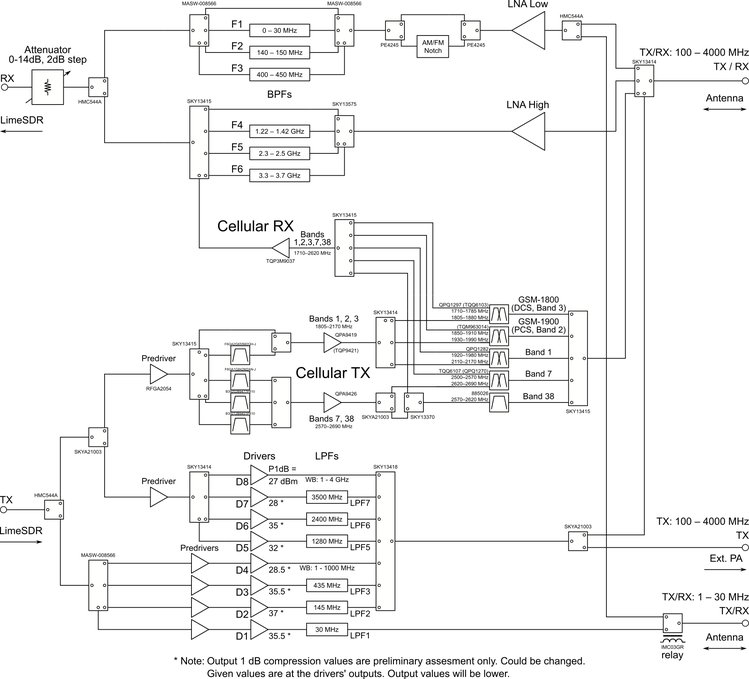
The LimeRFE is intended to work as an RF frontend for the LimeSDR family, although it can work coupled with any other SDR or conventional radio. As such, it has power amplifiers, filters and LNAs designed to cover the huge frequency range of these SDRs. It is designed to cover all the Amateur radio bands from HF up to 9cm, and a few cellular bands.

As anyone will know, designing broadband RF hardware is often quite difficult or expensive (Amateur radio amplifiers and LNAs are usually designed for a single band), so packing all this into a single unit is a considerable feat. The output power on most bands is around a couple watts, which is already enough for many experiments and applications. The block diagram of the LimeRFE can be seen below.

LimeRFE block diagram

In this post I show a brief overview of the LimeRFE and demonstrate its HF transmission capabilities by showing a WSPR transmitter in the 10m band, using a LimeSDR as the transmitter.

Measuring a mains choke with Hermes-Lite VNA

I have made a mains choke for my HF station, following Ian GM3SEK’s design, which involves twisting the three mains wires together and passing as many turns as possible through a Fair-Rite 0431177081 snap-on ferrite core. I wanted to measure the choke’s impedance to get an idea of its performance, so I’ve used my Hermes-Lite 2.0 beta2 in VNA mode.