Maia SDR DDC

I have implemented an FPGA DDC (digital downconverter) in Maia SDR. Intuitively speaking, a DDC is used to select a slice of the input spectrum. It works by using an NCO and mixer to move to the centre of the slice to baseband, and then applying low-pass filtering and decimation to reduce the sample rate as desired (according to the bandwidth of the slice that is selected).

At the moment, the output of the Maia SDR DDC can be used as input for the waterfall display (which uses a spectrometer that runs in the FPGA) and the IQ recorder. Using the DDC allows reaching sample rates below 2083.333 ksps, which is the minimum sample rate that can be used with the AD936x RFIC in the ADALM Pluto (at least according to the ad9361 Linux kernel module). Therefore, the DDC is useful to monitor or record narrowband signals. For instance, using a sample rate of 48 ksps, the 400 MiB RAM buffer used by the IQ recorder can be used to make a recording as long as 36 minutes in 16-bit integer mode, or 48 minutes in 12-bit integer mode. With such a sample rate, the 4096-point FFT used in the waterfall has a resolution of 11.7 Hz.

In the future, the DDC will be used by receivers implemented on the FPGA, both for analogue voice signals (SSB, AM, FM), and for digital signals. Additionally, I also have plans to allow streaming the DDC IQ output over the network, so that Maia SDR can be used with an SDR application running on a host computer. It is possible to fit several DDCs in the Pluto FPGA, so this would allow tuning independently several receivers within the same window of 61.44 MHz of spectrum. In the rest of this post I describe some technical details of the DDC.

In general, a DDC is formed by two elements: an NCO and mixer that performs frequency shifting, and a decimating low-pass filter. The mixer can be implemented as a CORDIC, or as a complex multiplier and a lookup table for the complex exponential (or a real sinusoid) function. The CORDIC requires only additions and subtractions, but it needs over a dozen stages to obtain a result that is accurate enough. The stages are implemented as a pipeline, so the CORDIC uses a reasonably large amount of logic. The advantage is that it doesn’t require any multipliers.

The lookup table approach requires multipliers to implement the complex multiplication. In Xilinx 7000 series and UltraScale+ FPGAs, complex multiplication can be done with DSP48Es. Either 3 DSP48Es can be used to implement a complex product that runs at one clock cycle per sample, or a single DSP48E can calculate a complex product using 3 clock cycles per sample. The lookup table can be implemented with BRAMs, but there are also all sorts of tricks to reduce the size of the table at the cost of additional logic (for instance, think about approximating the sine function piecewise with polynomials of low order).

These two approaches are commonly used, and often the factor that decides which approach is best for some particular application is how many DSPs and BRAMs versus logic a particular FPGA has. In the case of Maia SDR, I’m using the complex product approach with a single DSP48E that runs at 187.5 MHz (so it always has at least 3 clock cycles per sample, even at the maximum sample rate of 61.44 Msps), and a 1024-entry lookup table for the complex exponential with 18-bit resolution for the real and imaginary parts. This table fits in a single 36 kb BRAM.

For the low-pass filtering and decimation, the most common approach is to use a CIC filter followed by some FIR filters with a fixed design. For instance, these FIR filters can be either two or three half-band filters, each of which can be bypassed, or it can be a single decimate-by-4 or decimate-by-2 FIR filter with compensation for the CIC response, or a combination of these ideas. The motivation behind this approach is that the CIC filter does not require multipliers and it has a simple design that can be set to any decimation ratio at runtime (as long as the decimation doesn’t exceed the maximum value for which the bit growth in the datapath has been designed). The disadvantage of the CIC filter is that its passband is not flat, and the stopband rejection isn’t great either. The FIR filters following the CIC select only the central part of the CIC output spectrum. In this part, the spectrum is flatter and the stopband rejection of aliases is better. If the FIR filters implement compensation, the output passband is made even flatter. The downside of using a CIC is that odd decimation factors do not work well, because the FIR filters must be bypassed. For good results, the decimation factor needs to be even, or better, a multiple of 4, or even better, a multiple of 8 (if there are 3 half-band filters).

In the Maia SDR DDC, I have decided to follow a different approach, based on the paper Optimum FIR Digital Filter Implementations for Decimation, Interpolation, and Narrow-Band Filtering, by Crochiere and Rabiner. I first learned about this paper from Youssef Touil from Airspy. It is an old paper from the 70s where the authors argue that a good way to design a decimating FIR filter that performs a minimal number of multiplications per input sample is to perform two or three stages of decimating FIR filters. The first stage runs at the full input sample rate, but can have a rather large transition bandwidth, so it doesn’t need many coefficients. The final stage is the one with a narrow transition bandwidth, which requires many coefficients. However, since it runs at a reduced sample rate, the number of multiplications per input sample is not so high. This idea is also present throughout the book Multirate Signal Processing for Communications Systems, by fred harris.

I haven’t seen an FPGA DDC implementation based on this idea before. I think that the reason for this is that the design is more complicated that the one based on the CIC. Changing the decimation factor of a CIC is as easy as changing the period of a counter that controls the output strobe of the CIC. On the other hand, changing the decimation factor of a cascade of 3 FIRs as in the Crochiere and Rabiner paper requires choosing how the decimation shall be split between the FIRs in the cascade, and designing new FIR coefficients. Rather than using a fixed FIR implementation, a programmable FIR implementation whose coefficients and decimation ratio can be changed at runtime is needed.

Nevertheless, I have followed the FIR cascade idea in Maia SDR. The main reason is that I wanted to do something innovative instead of reimplementing an approach that is already present in open source SDRs such as the USRPs and the Hermes. Additionally, I think that the FIR cascade can be a better solution than the CIC DDC in some situations, so I wanted to test how well a FIR cascade implementation works in the real world. The main motivation for using a FIR cascade is avoiding the CIC, which uses a considerable amount of logic. The reasoning is that even with the CIC some FIRs are needed, and these will use DSPs. By designing a FIR-only DDC perhaps a few more DSPs are needed, but all the logic of the CIC is saved.

In think that current Xilinx FPGAs have comparatively more DSPs than logic. A look at the Zynq 7000 product selection guide shows that the ratio between the number of LUTs and number of DSPs for Zynq 7000 devices ranges between 190 and 290 LUTs/DSP, except for the Zynq 7100, which has a very large amount of DSPs and gets a ratio of 137 LUTs/DSP. UltraScale+ FPGAs are even more DSP-dense. The MPSoC product selection guide gives that the ratio for CG devices is around 170-190 LUTs/DSP for the ZU3CG and smaller devices, and around 90-130 LUTs/DSP for larger devices. For many kinds of signal processing algorithms, the amount of work you can do with one DSP is much larger than what you can do with 100 or 200 LUTs, specially taking into account the fact that DSPs can usually be run at much higher clock frequencies than logic. So for me, with today’s DSP-dense FPGAs, in general it is better to use signal processing algorithms and implementations that make heavy use of DSPs instead of using more traditional approaches that were designed to avoid using multipliers. Of course, for any concrete application the situation will be more nuanced than this, since if absolutely everything is done with DSPs, then the DSPs will quickly become the resource that limits what can be fitted in the FPGA.

The Maia SDR DDC has 3 stages of FIR filters. The coefficients and decimation factor of each FIR are fully programmable at runtime, and each stage except for the first can be bypassed. The FIRs are clocked with a 187.5 MHz clock, so there are at least 3 clock cycles per input sample. The first and third stages are identical. They have 2 DSPs for the real part and 2 DSPs for the imaginary part. This means that the first stage can perform up to 6 multiplications per output sample at the highest input sample rate of 61.44 Msps. The maximum number of coefficients supported by these FIRs is 256. The second stage is smaller: it uses only one DSP for the real part and one DSP for the imaginary part, and the maximum number of coefficients is 128. This is done because I evaluated several FIR cascade designs following the paper of Crochiere and Rabiner and found that the second stage can usually be smaller. The first stage often needs to perform nearly 6 multiplications per output sample, so it needs to have 4 DSPs. The last stage often needs a long FIR to achieve a narrow transition bandwidth, and to realize this FIR it is often necessary to use 4 DSPs as well. But the second stage doesn’t have any of these more strict requirements, so it can be simpler.

Each FIR filter is implemented with a polyphase architecture. This makes it relatively easy to address the samples and coefficients, which are stored in BRAMs. However, it means that we don’t take advantage of the symmetry of the FIR coefficients. It would be interesting to compare this with an implementation that uses the FIR coefficient symmetry to reduce the number of multiplications (and hence the number of DSPs needed). This implementation would require a more complex addressing logic.

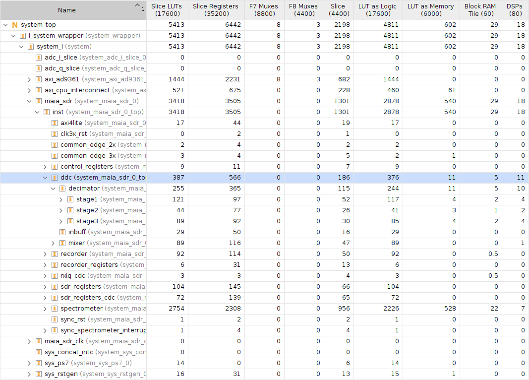
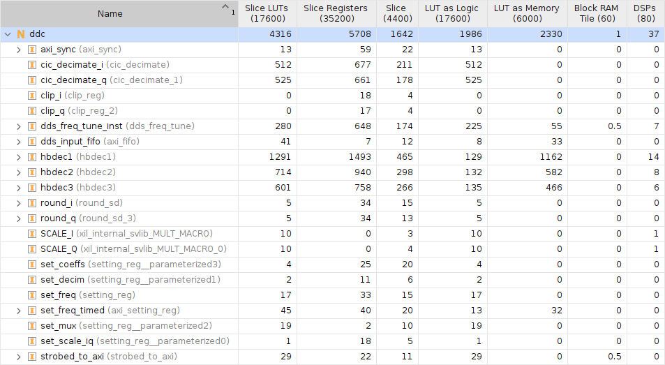
The following figure shows the resource utilization of the Maia SDR Pluto image, with the DDC divided by submodules. The FIR decimator needs 10 DSPs, as discussed above, and another DSP is used in the mixer. Besides this, the FIRs need 5 BRAM to store the coefficients and samples. There is another BRAM required to store the complex exponential for the mixer, but Vivado has placed this in the maia_sdr module directly, so really the DDC needs 6 BRAM. Less than 400 LUTs are used by the DDC.

As a comparison, I have done an out-of-context synthesis and implementation of the RFNoC DDC used in the Ettus USRP 300 series (when doing this, I have targetted the same Zynq 7010 FPGA that is used in the Pluto). The RFNoC DDC has a CIC followed by three half-band FIRs, which can be bypassed. This comparison is quite far from being fair, in part because the capabilities of the DDCs are quite different. There are some decimation factors which work well with the RFNoC DDC but don’t work well with the Maia SDR DDC. For instance, decimation by either 2, 4 or 8 works very well with the RFNoC DDC, but it doesn’t work well with the Maia SDR DDC, because its FIR cascade design relies on having the first stage perform a moderate amount of decimation so that the following stages can implement longer filters with few DSPs. Thus, small decimation factors and factors which are prime do not work well with this design. On the other hand, the Maia SDR DDC works quite well for odd composite large decimation ratios, and the RFNoC DDC doesn’t because i can’t use its half-band FIRs.

Something to keep in mind when comparing these two designs is that the Maia SDR DDC design needs a clock with at least 3 clock cycles per input sample, while the RFNoC DDC is designed to run at one clock cycle per input sample. So to try to compare DSP usage directly, we should count each Maia SDR DDC DSP as 3 DSPs. If we do this, the Maia SDR DDC requires 33 DSPs, while the RFNoC DDC requires 37. The DSP usage is similar, but the Maia SDR DDC has saved all the logic needed for the CIC, which is around 1000 LUTs.

Regarding DSP usage, note that the RFNoC DDC uses 2 DSPs to perform a final output scaling, which is mainly needed because CIC gain depends on the decimation factor. The Maia SDR DDC doesn’t need this output scaling, not only because it doesn’t have a CIC, but also because since it has programmable FIR coefficients, the scaling can be applied to the coefficients. Something else to note is that the mixer in the RFNoC DDC uses 7 DSPs, instead of the one (which should be counted as 3) in the Maia SDR DDC. This is because it has a complex multiplier that uses 4 DSPs instead of 3 (probably because it performs the complex product in the naïve way instead of using one of the usual tricks to compute it with only 3 real products), and because the complex exponential is generated with 0.5 BRAMs and 3 DSPs instead of 1 BRAM as in Maia SDR.

Even taking into account these differences, for me the conclusion is that the Maia SDR DDC design uses slightly more DSPs for the FIRs than a DDC based on a CIC, but it saves all the logic required for the CIC. Therefore, I think that this FIR cascade design can be quite competitive with the usual design based on a CIC, and can be better in many cases, specially when the decimation factors are large composite numbers.

A cascade of programmable FIR filters needs to go hand in hand with some software that can be used to design these FIR filters, computing the coefficients on the fly as the decimation ratio is changed. For this, I have implemented the Parks-McClellan (Remez) algorithm in Rust, about which I spoke last month. Besides the FIR filter design algorithm itself (which could be Parks-McClellan, the window method, or any other), the Crochiere and Rabiner FIR cascade requires to determine how the total decimation ratio is split over the FIR stages. The total number of multiplications per input sample depends on this split. This not only impacts power consumption, but also whether a filter is realizable by the FPGA implementation, because it doesn’t exceed the maximum number of multiplications and FIR length for each stage.

One possible approach to choose the decimation ratio split is to compute the design for each of the possible splits and then choose the one which is optimal according to a certain metric, such as the number of multiplications per input sample. However, this is very time consuming. Our design requirements are the stopband attenuation, the passband ripple, and the cutoff frequencies for the passband and stopband. However, the Parks-McClellan algorithm needs to be run for a fixed number of coefficients. Therefore, it is necessary to run the algorithm multiple times to find the smallest number of coefficients that satisfies the requirements (an alternative idea would be to run Parks-McClellan just once for the maximum number of coefficients that can be implemented by the FPGA for some particular input sample rate and decimation split configuration, but I haven’t experimented much with this idea).

In order to perform the design faster, the formulas from the paper Accurate estimation of minimum filter length for optimum FIR digital filters, by Ichige, Iwaki and Ishii, are used to estimate the number of coefficients that the Parks-McClellan FIR will have. The split is chosen as the one which gives the minimum number of multiplications per input simple if the FIR lengths are chosen as indicated by this estimate. Therefore, this choice is only a guess of what is the best split, but it is usually the correct guess, or one that performs only slightly worse that the guess. The estimation is also used as a starting point to determine the shorter FIR length that can be used.

The design requirements for the DDC FIR cascade can be set with the Maia SDR web user interface. These are the transition bandwidth, the passband ripple, the stopband attenuation, and whether the stopband should have a 1/f response. The transition bandwidth is given as the fraction of the output spectrum that is affected by the filter skirts and aliasing. For instance, a value of 0.05 means that 5% of the output spectrum has these problems, but the central 95% of the output spectrum is flat and has no aliasing.

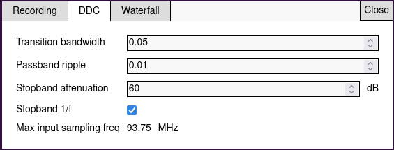
The design obtained using Parks-McClellan and loaded into the FPGA implementation has a certain maximum input sample rate that depends on these settings and the desired decimation factor. In some cases, the maximum input sample rate can be smaller than 61.44 Msps, which is the maximum output sample rate of the AD9361. This means that if we want to use this decimation ratio with an input sample rate of 61.44 Msps, we will need to sacrifice some of the filter performance, for instance by making the transition bandwidth larger, or the stopband attenuation smaller. This gives the user a very flexible way of configuring the FIR filters depending on the intended use case.

Designing the FIR filters by running Parks-McClellan on the Zynq ARM CPU takes a few seconds for large decimation ratios (on the order of 1000). I think this is acceptable for most applications. If a faster response time was necessary, it would be possible to have a cache of previously computed design, and/or a database of precomputed designs.

The web user interface configures the DDC by sending a PUT HTTP request to the API URL /api/ddc/design. The PUT request contains a JSON object that lists the decimation factor, the mixer frequency, and the requirements shown above (transition bandwidth, etc.). Third-party applications can also use this API. There is also a lower-level API in the URL /api/ddc/config. This allows sending a PATCH or PUT request with the decimation factor and the list of coefficients for each FIR in the cascade. In this way, third-party applications can use the FPGA DDC more freely by loading FIR filter designs computed in a different way. The list of FIR filters coefficients that are currently loaded can be queried with a GET request on /api/ddc/config. Among other things, this can be used by a third-party application to obtain the FIR filters that have been computed with Parks-McClellan, and do things such as plotting their frequency response.