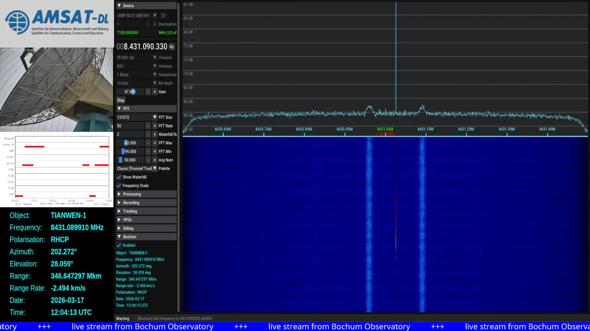
The signal strength looks completely normal, as evidenced by the spectrum plot shared in the announcement.
Screenshot of Tianwen-1 reception in Bochum shared by AMSAT-DL
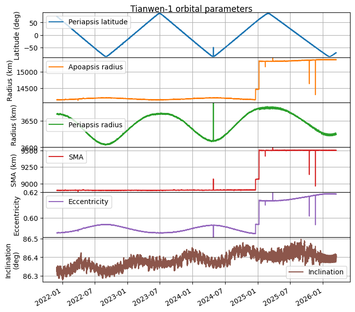
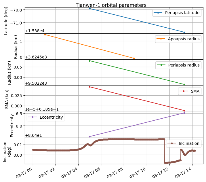
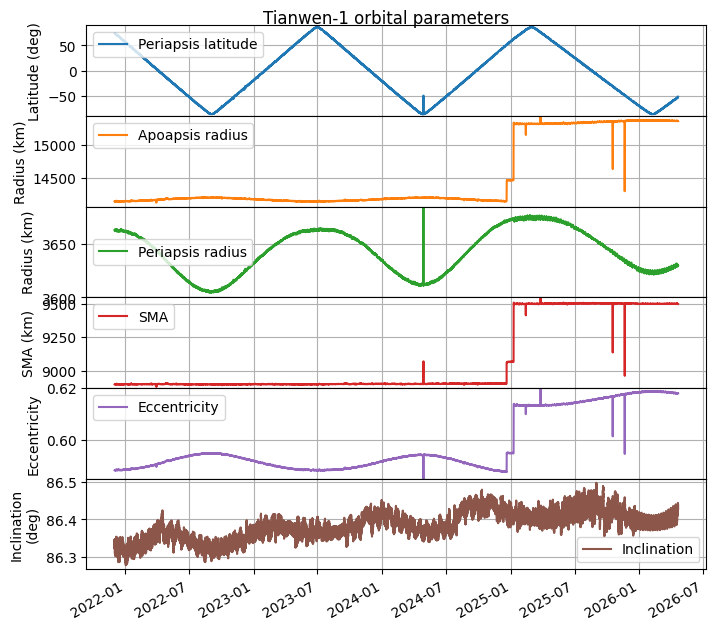
Telemetry containing state vectors was decoded between 2026-03-17 11:34 and 14:16 UTC. I have updated my plot of orbital parameters to include this new information. The period between 2025-12-23 and 2026-03-17 corresponds to a propagation with GMAT of the last telemetry received in 2025. The end of the plot corresponds to the telemetry received in 2026-03-17.
We can see that the orbit has remained the same, and there have been no manoeuvres during this period. A zoomed in version to the end of the plot shows that there is basically no jump in the orbital parameters. There is a tiny jump in the inclination as the new telemetry is received, but that is all.
So far the reasons why Tianwen-1 has apparently not transmitted telemetry to Earth for almost 3 months remain unknown.
Yesterday, AMSAT-DLpublished the news that they have been unable to receive any signals from Tianwen-1 with the 20 m antenna in Bochum since 2025-12-23. As you may know if you have been following my posts about Tianwen-1, AMSAT-DL has been using this antenna to receive and decode telemetry from Tianwen-1 almost every day since the beginning of the mission in 2020-07-23. The news about the lack of signal detected from Tianwen-1 over the last few months were hardly a secret, because AMSAT-DL runs a livestream of the signals received with the Bochum antenna 24/7, so anyone could look at the livestream and realize that Tianwen-1 was being observed but no signal was visible on the spectrum. However, now that the public has been made well aware of this fact, I can make some more comments about it. There has been no public communication from the Chinese space program regarding this, so the fate of Tianwen-1 is currently unknown.
During December 2025 and January 2026, there was a Mars conjunction, which means that Mars goes behind the Sun as seen from Earth. Communications with Mars orbiters cannot happen during this period of time. For instance, this news piece hints at NASA Mars missions not having contact between 2025-12-29 and 2026-01-16, which corresponds to a Sun-Earth-Mars angle (elongation) of 3º on 2025-12-29 and 1.8º on 2026-01-16, with the minimum elongation achieved on 2026-01-09. Therefore, it was completely expected that we would lose Tianwen-1’s signal during the conjunction period. Because the communications link to Earth does not work, spacecraft will usually not point their high gain antennas to Earth and even stop transmitting during this period. However, we expected to see Tianwen-1 back again after the conjunction, and we never did.
I have been using the telemetry decoded by AMSAT-DL, which includes the spacecraft state vectors, to keep track of the spacecraft orbit. I have been posting updates about any change that happens. The last one was the apoapsis raise on 2025-01-08. The lack of signals from Tianwen-1 sparked internal discussion about whether the spacecraft might have intentionally reentered some time around the conjunction period as a way of terminating the mission without leaving orbital debris. To analyse whether this could be possible, I have updated my orbit analysis to account for all the telemetry that has been received so far, up to 2025-12-22, which is when the last telemetry was decoded.
The result can be seen in the figure below. We see the apoapsis raises that happened during the end of 2024 and beginning of 2025. After that there have been no manoeuvres.
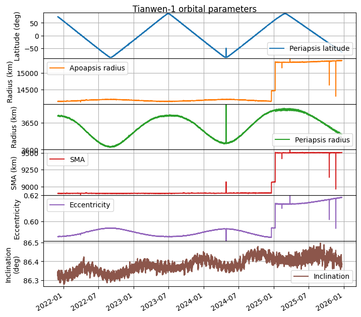
Since the plot above indicates that the periapsis radius would be going towards a minimum at the beginning of 2026 due to long-term periodic orbit perturbations, I propagated the last telemetry data we have forward with the goal of studying the impact of the larger apoapsis radius. The results are shown here. We note that the apoapsis radius minimum is now much higher than in the past, so the hypothesis of a reentry is unlikely unless a manoeuvre that we didn’t see in the telemetry has happened.
Back in November, I posted about the ESCAPADE Mars twin orbiter mission. I made a recording of the X-band telemetry with the Allen Telescope Array the day after launch, and I decoded the telemetry with GNU Radio. I made a preliminary analysis of the telemetry, showing that it contained a large number of log messages in ASCII. Shortly after writing this post, PistonMiner provided a deeper analysis of the telemetry, including a Github repository with some code and extracted data. She noticed that the CCSDS Space Packets, all of which belonged to the same APID 51, contained MAX simple telemetry frames in their payloads. Since MAX telemetry frames contain their own APIDs, this allowed separating the different types of telemetry data. Since seeing this, I wanted to go back and analyse again the telemetry to see what else I could find. Now I’ve finally had some time to do this. In this post I describe my new findings, as well as what PistonMiner originally discovered.
CSP is the Cubesat Space Protocol. It is a network protocol that was developed by Aalborg university, and is commonly used in cubesats, in particular those using GOMspace hardware. Initially the protocol allowed different nodes on a satellite to exchange packets over a CAN bus, but eventually it grew into a protocol that spans a network composed by nodes in the satellite and the groundstation that communicate over different physical layers, including RF links.
Recently I have been working on a project that involves CSP. To measure network performance and debug network issues, I have written some tooling in Rust, as well as a Wireshark dissector in Lua. The Rust tooling is an implementation from scratch and doesn’t use libcsp. Now I have open sourced these tools in a csp-tools repository and csp-tools Rust crate. In this post I showcase how the tools work.
In my previous post I decoded a transmission from a V16 beacon. The V16 beacon has mandatorily replaced warning triangles in Spain in 2026. It is a device that contains a strobe light and an NB-IoT modem that sends its GNSS geolocation using the cellular network. It is said that the beacon first transmits is geolocation 100 seconds after it has been powered on, and then it transmits it again every 100 seconds. In that post I recorded one of those transmissions done after the beacon had been powered on for a few minutes and I decoded it by hand. I showed that the transmission contains a control plane service request NAS message that embeds a 158 byte encrypted message, which is what presumably contains the geolocation and other beacon data.
In that post I couldn’t show how the beacon connects to the cellular network and sets up the EPS security context used to encrypt the message, since that would have happened some minutes before I made the recording. I have now made a recording that contains both the NB-IoT uplink and the corresponding NB-IoT downlink and starts before the V16 beacon is switched on. In this post I show the contents of the uplink recording.
The V16 beacon is a car warning beacon that will mandatorily replace the warning triangles in Spain starting in 2026. In the event of an emergency, this beacon can be magnetically attached to the roof of the car and switched on. It has a bright LED strobe light and a connection to the cellular network, which it uses to send its GNSS position to the DGT 3.0 cloud network (for readers outside of Spain, the Spanish DGT is roughly the equivalent of the US DMV). The main point of these beacons is that placing warning triangles far enough from a vehicle can be dangerous, while this beacon can be placed without leaving the car.
There has been some criticism surrounding the V16 beacons and their mandatory usage that will start in January 2026, both for economical and implantation roadmap reasons, and also for purely technical reasons. The strobe light is so bright that you shouldn’t look at it directly while standing next to the beacon (which makes it tricky to pick it up and switch it off), but I have heard that it is not so easy to see in daylight from several hundreds of meters away.
The GNSS geolocation and cellular network service is also somewhat questionable. I purchased a V16 beacon from the brand NK connected (certificate number LCOE 2024070678G1), for no reason other than the fact that it was sold in a common supermarket chain. The instructions in the box directed me to the website validatuv16.com for testing it. In this website you can register the serial number or IMEI of your beacon and your email. Then you switch on the beacon. After 100 seconds the beacon should send a message to the DGT network, and then periodically every 100 seconds. This test service is somehow subscribed to the DGT network, and it sends you an email that contains the message data (GNSS position and battery status) when the DGT network receives it. This is great, but there is no test mode or anything that declares that you are using the beacon just for testing purposes. They only say that you should not leave the beacon on for much longer than what it takes you to receive the email, to avoid the test being mistaken for a real emergency. The fact that the test procedure for this system is literally the same as the emergency procedure is a red flag for me. Additionally, this beacon only includes cellular data service for 12 years, and it is not clear what happens after that.
Technical shortcomings aside, my main interest is how the RF connection to the DGT network works. The beacon I bought has a logo in the box saying that it uses the Orange cellular network. When I tested it, after receiving the confirmation email from the test service, I used a Pluto SDR running Maia SDR and quickly found that the beacon was transmitting NB-IoT on 832.3 MHz. I made a recording of one of the periodic transmissions. In this post I analyse and decode the recording.
A few days ago I was doing some refactoring of my galileo-osnma project. This is a Rust library that implements the Galileo OSNMA (open service navigation message authentication) system. The library includes a demo that runs in a Longan nano GD32VF103 RISC-V microcontroller board. The purpose of this demo is to show that this library can run on small microcontrollers. My refactoring was in principle a simple thing: I was mainly organizing the repository as a Cargo workspace, and unifying the library and some supporting tools into the same crate. However, after the refactor, users reported that the Longan nano software was broken. It would hang after processing some messages. This post is a collection of notes about how I investigated the issue, which turned out to be related to stack usage.
The Lunar GNSS Receiver Experiment (LuGRE) is a NASA and Italian Space Agency payload that flew in the Firefly Blue Ghost Mission 1 lunar lander. An overview of this experiment can be found in this presentation. The payload contains a Qascom GPS/Galileo L1 + L5 receiver capable of both real time positioning and raw IQ recording, and a 16 dBi high-gain antenna that was pointed towards Earth. For decades the GNSS community has been talking about using GNSS in the lunar environment, and LuGRE has been the first payload to actually demonstrate this concept.
The LuGRE payload ran a total of 25 times over the Blue Ghost mission duration, starting with a commissioning run on 2025-01-15 a few hours after launch and ending with a series of 9 runs on the lunar surface between 2025-01-03 (the day after the lunar landing) and 2025-01-16 (end of mission after lunar sunset). Back in October 15, the experiment data was published in Zenodo in the dataset Lunar GNSS Receiver Experiment (LuGRE) Mission Data. This dataset includes some short raw IQ recordings, as well as output from the real time GNSS receiver (raw observables, PVT, ephemeris and acquisition data). Since I have some professional background implementing high-sensitivity GNSS acquisition algorithms and I find this experiment quite interesting, I decided to do some data analysis, mainly of the raw IQ data.
The initial results of the experiment were presented on September 11 in the ION GNSS+ 2025 conference in a talk titled Initial Results of the Lunar GNSS Receiver Experiment (LuGRE). This talk is only available to registered ION attendees. As I don’t want to resort to my network to scrounge some ION paper credits (which is how proceedings are usually downloaded from the ION website), I haven’t seen anything about this talk besides the abstract. It is quite possible that something of what I will mention here was already presented in this talk. This is what we get as a society for not doing science in a completely public and open way. However, it’s interesting that this also makes my analysis less likely to be biased. I’ve just downloaded some raw IQ data and started looking at it with only basic context about the instrument that produced it and how it was run.
For a first analysis, I have implemented a high-sensitivity acquisition algorithm for the GPS L1 C/A signal in CUDA. I have run this on all the 20 L1 IQ recordings that are available. In this post I present the algorithm and the results.
ESCAPADE is a twin spacecraft mission that will study the Mars magnetosphere. The science mission is led by UC Berkeley Space Sciences Laboratory and the spacecraft buses were built by Rocket Lab. It was launched on November 13 on the second Blue Origin New Glenn mission NG-2. The spacecraft will spend a year around the Earth-Sun L2 Lagrange point before falling back to Earth for a powered gravity assist that will place them on Hohmann transfer orbit to Mars as the “launch window” to Mars opens. These are the first spacecraft to fly this kind of trajectory.
I have published a new Python package called sigmf-toolkit. It is intended to be a collection of Python tools to work with SigMF files. At the moment it only contains two tools, but I plan on adding more tools to this package as the needs arise. These tools are:
gr_meta_to_sigmf. It converts a GNU Radio metadata file with detached headers to a SigMF file. At the moment it is really simple, and it doesn’t handle capture discontinuities.
sigmf_pcap_annotate. This tool parses a PCAP file using Scapy and it adds annotations to a SigMF file for each packet in the PCAP file.
I find this sigmf_pcap_annotate tool quite useful when comparing side by side a SigMF file in Inspectrum and a PCAP file in Wireshark to debug issues with digital communications systems. In this post I showcase how this tool can be used.