Back in May, I spoke about the future collision of DSLWP-B with the lunar surface. It would happen on July 31, thus putting and end to the mission. Now that the impact date is near, I have run again the calculations with the latest ephemeris in order to have an accurate simulation of the event.
The ephemeris I’m using consist of a Moon centred ICRF Keplerian state vector which has been shared by Wei Mingchuan BG2BHC. In GMAT, this state vector is as follows:
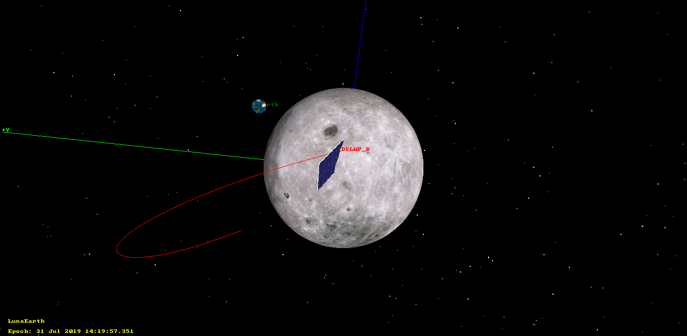
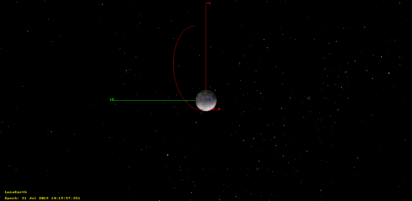
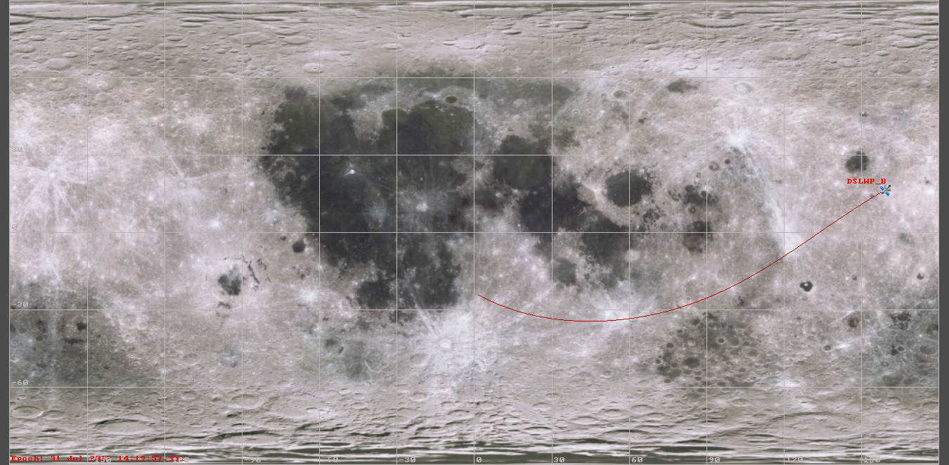
Using this GMAT script, I have obtained that the impact will happen on 2019-07-31 14:19:57 UTC, near Mare Moscoviense, in the lunar far side. This result is quite close to the calculations I did in May, which predicted an impact at 14:47 UTC.
The images below show the impact simulation in GMAT. Since the impact happens on the far side of the Moon, it will not be visible from Earth. There is an activation of the Amateur payload onboard DSLWP-B for 2019-07-31 13:24 to 15:24 UTC. The satellite will hide behind the Moon around 14:08 UTC. If the Moon was not solid, DSLWP-B would reappear around 14:35 UTC. The absence of radio signals after this moment will confirm that the impact has occurred.
DLSWP-B impact orbit in GMAT (view of Earth and Moon)DSLWP-B impact orbit in GMAT (top view)Ground track and location of DSLWP-B impact in GMAT
SkyFox Labs is having some trouble identifying the TLE corresponding to their Lucky-7 cubesat. The satellite was launched on July 5 in launch 2019-038 and a good match among the TLEs assigned to that launch has not being found yet. Over on Twitter, Cees Bassa has analyzed some SatNOGS observations and he says that NORAD ID 44406 seems the best match. However, this TLE has already been identified by Spire as belonging to one of their LEMUR satellites.
Fortunately, Lucky-7 has an on-board GPS receiver, and the team has been collecting position data recently. This data can be used to match a TLE to the orbit of the satellite, and indeed is much more accurate than the Doppler curve, which is the usual method for TLE identification.
Jaroslav Laifr, from the Lucky-7 team, has sent me the data they have collected, so that I can study it to find a matching TLE. The study is pretty simple to do with Skyfield. I have obtained the most recent TLEs for launch 2019-038 from Space-Track and computed the RMS error between each of the TLEs and the GPS measurements. The results can be seen in this Jupyter notebook.
The best match is NORAD ID 44406, with an RMS error of 8.7km. The second best match is NORAD ID 44404 (which is what SatNOGS has been using to track Lucky-7), with an RMS error of 51.3km. Most other objects have an error larger than 100km.
Therefore, my conclusion is clear. It is very likely that Spire misidentified NORAD ID 44406 as belonging to LEMUR 2 DUSTINTHEWIND early after the launch, when the different objects hadn’t drifted apart much. NORAD ID 44406 is a good match for Lucky-7. It will be interesting to see what Spire says in view of this data.
In May 25, the Moon passed through the beam of my QO-100 groundstation and I took the opportunity to measure the Moon noise and receive the Moonbounce 10GHz beacon DL0SHF. A few days ago, in July 22, the Moon passed again through the beam of the dish. This is interesting because, in contrast to the opportunity in May, where the Moon only got within 0.5º of the dish pointing, in July 22 the Moon passed almost through the nominal dish pointing. Also, incidentally this occasion has almost coincided with the 50th anniversary of the arrival to the Moon of Apollo 11, and all the activities organized worldwide to celebrate this event.
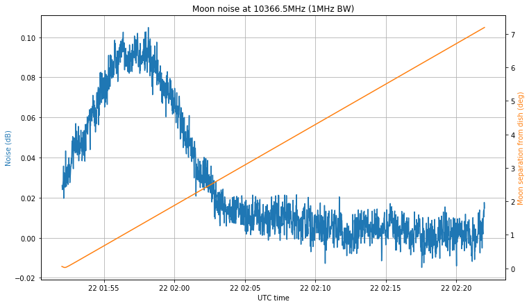
The figure below shows the noise measurement at 10366.5GHz with 1MHz and a 1.2m offset dish, compared with the angular separation between the Moon and the nominal pointing of the dish (defined as the direction from my station to Es’hail 2). The same recording settings as in the first observation were used here.
The first thing to note is that I made a mistake when programming the recording. I intended to make a 30 minute recording centred at the moment of closest approach, but instead I programmed the recording to start at the moment of closest approach. The LimeSDR used to make the recording was started to stream one hour before the recording, in order to achieve a stable temperature (this was one lesson I learned from my first observation).
The second comment is that the maximum noise doesn’t coincide with the moment when the Moon is closest to the nominal pointing. Luckily, this makes all the noise hump fit into the recording interval, but it means that my dish pointing is off. Indeed, the maximum happens when the Moon is 1.5º away from the nominal pointing, so my dish pointing error is at least 1.5º. I will try adjust the dish soon by peaking on the QO-100 beacon signal.
The noise hump is approximately 0.085dB, which is much better than the 0.05dB hump that I obtained in the first observation. It may not seem like much, but assuming the same noise in both observations, this is a difference of 2.32dB in the signal. This difference can be explained by the dish pointing error.
The recording I have made also covers the 10GHz Amateur EME band, but I have not been able to detect the signal of the DL0SHF beacon. Perhaps it was not transmitting when the recording was made. I have also arrived to the conclusion that the recording for my first observation had severe sample loss, as it was made on a mechanical hard drive. This explains the odd timing I detected in the DL0SHF signal.
The next observation is planned for October 11, but before this there is the Sun outage season between September 6 and 11, in which the Sun passes through the beam of the dish, so that Sun noise measurements can be performed.
Lucky-7 is a Czech Amateur 1U cubesat that was launched on July 5 together with the meteorological Russian satellite Meteor M2-2 and several other small satellites in a Soyuz-2-1b Fregat-M rocket from Vostochny. The payload it carriers is rather interesting: a low power GPS receiver, a gamma ray spectrometer and dosimeter, and a photo camera.
It transmits telemetry in the 70cm Amateur satellite band using 4k8 FSK with an Si4463 transceiver chip. Additional details about the signal can be found here.
After some work trying to figure out the scrambler used by the Si4463, I have added a decoder for Lucky-7 to gr-satellites. This post shows some of the technical aspects of the decoder.
During this week, the Amateur payload of DSLWP-B was active during the following slots:
14 Jul 19:00 to 21:00
15 Jul 12:00 to 14:00
17 Jul 04:40 to 06:50
18 Jul 20:50 to 22:50
20 Jul 14:20 to 16:20
21 Jul 05:30 to 07:30
Among these, the Moon was visible from Europe only on July 14, 18 and 21, so Dwingeloo only observed these days, which were mainly devoted to the download of SSDV images of the lunar surface. As usual, the payload took an image automatically at the start of each slot, so some of the slots were used for autonomous lunar imaging, even though no tracking was made from Dwingeloo.
This post is a detailed account of the activities done with DSLWP-B during the third week of July.
During this week, the Amateur payload of DSLWP-B has been active on the following slots:
2019-07-09 12:30 to 14:30 UTC
2019-07-10 13:50 to 15:50 UTC
2019-07-12 02:00 to 04:00 UTC
2019-07-12 16:30 to 18:30 UTC
In these activations, the last remaining image of the eclipse was downloaded. Also, images of the lunar surface as well as stars have been taken and downloaded. This post is a summary of the activities made with DSLWP-B over the week.
Now that the DSLWP-B eclipse images have become widespread, appearing even in some newspapers, I have taken the time to identify the features of the lunar surface that can be seen in two of the images. As with any Earth and Moon pictures of DSLWP-B, the part of the Moon that can be seen in these images belongs to the far side, with longitudes of approximately 100º E and 100º W (the division between the near side and the far side happens at 90º E and 90º W, and 0º is the middle of the near side).
I have compared the images with a simulation of the camera view done in GMAT. Using this simulation as a reference and these lunar surface maps as well as Google Moon, I have labelled the features that are visible in the images. The 4K lunar surface map from Celestia Motherlode has been used in GMAT, instead of the default, lower resolution map.
Occultation entry
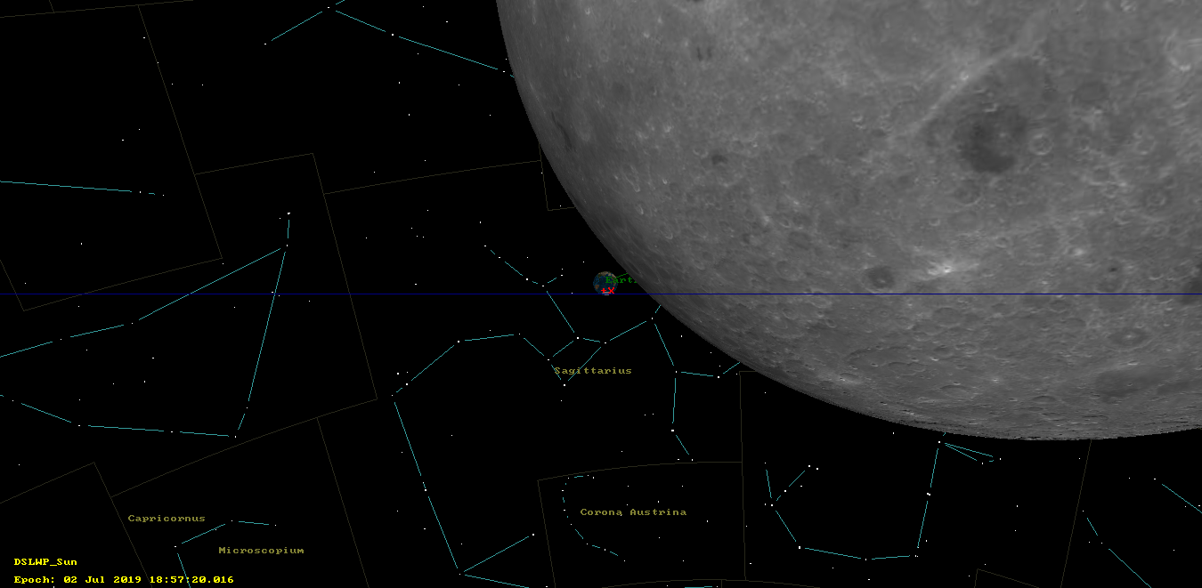
The figure below shows the GMAT camera view simulation for one of the images taken as DSLWP-B was hiding behind the Moon. The field of view in this figure is much larger than the field of view of the DSLWP-B Inory eye camera. The up direction is the normal to DSLWP-B’s orbit around the Sun (defined as the plane containing the position and velocity vectors with DLSWP-B with respect to the Sun). Therefore, it points approximately towards the north pole. DSWLP-B is moving towards the upper right corner of this image.
GMAT camera view simulation for image 0xE2
The figure belows shows the ground track view. The satellite has crossed the near side and is now starting to orbit over the far side, soon becoming hidden behind the Moon.
GMAT ground track view for image 0xE2
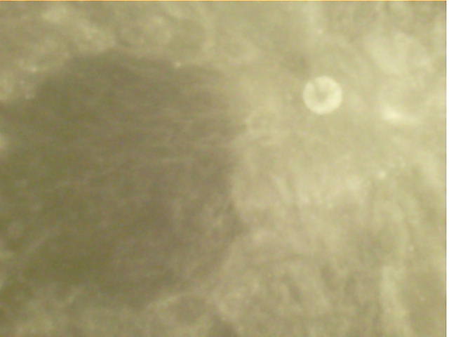
Image 0xE2, taken on 2019-07-02 18:57:20 is shown below. The image has been rotated to match the orientation of the GMAT camera view simulation.
Image 0xE2, rotated
The craters that are visible in this image are labeled in the figure below. These belong to the Mare Australe region, and several well known craters such as Jenner and Lamb can be seen.
Image 0xE2, rotated and labelled
Tammo Jan Dijkema has done a similar exercise with image 0xE3, which was taken a minute after the image shown above. DSLWP-B has moved towards the upper right corner of the image, so that a larger portion of the lunar surface is visible.
Here's the solar eclipse imaged from lunar orbit again, now with some lunar features labeled. These are of course all features on the far side of the Moon. pic.twitter.com/zMY9cxSgZ4
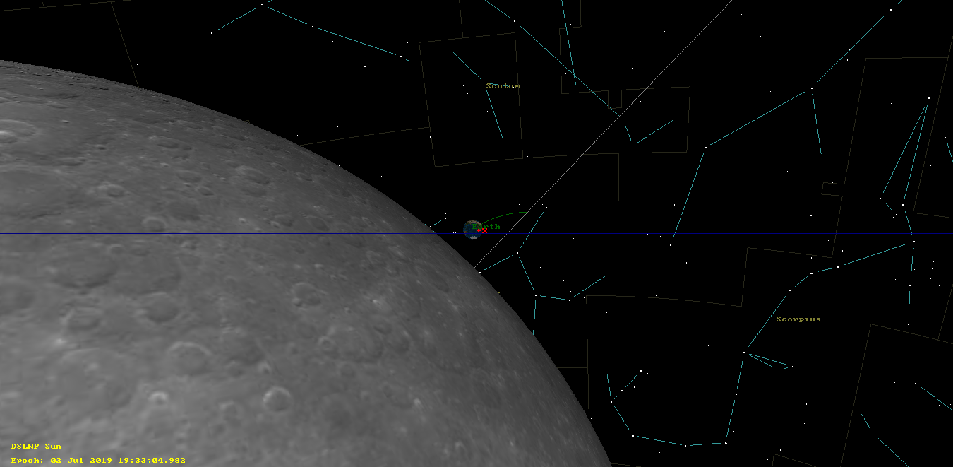
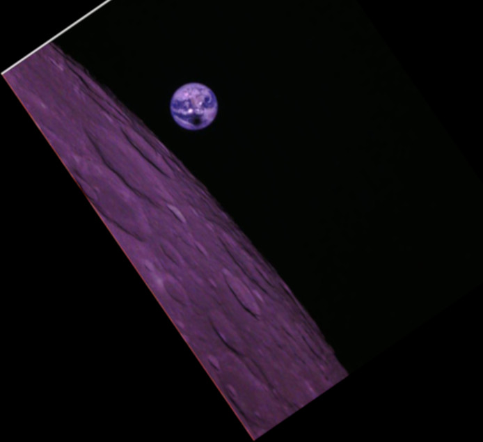
The figure below shows the GMAT camera view simulation corresponding to image 0xE5, which was taken shortly after DSLWP-B exited the occultation, so that the Earth was visible again.
GMAT camera view simulation for image 0xE5
Below we see the ground track corresponding to this image. The satellite has crossed the far side of the Moon in a south to north direction and soon will cross over to the near side.
GMAT ground track view for image OxE5
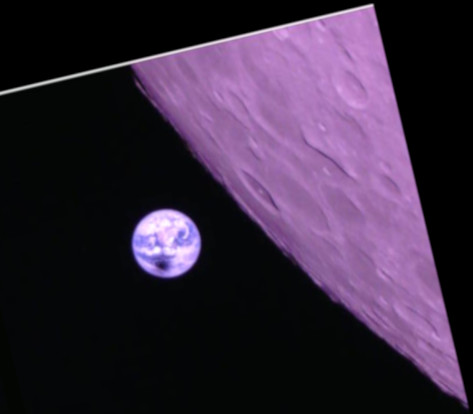
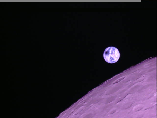
The figure below is image 0xE5, which was taken on 2019-07-02 19:33:05. It has been rotated to match the orientation of the GMAT simulation.
Image 0xE5, rotated
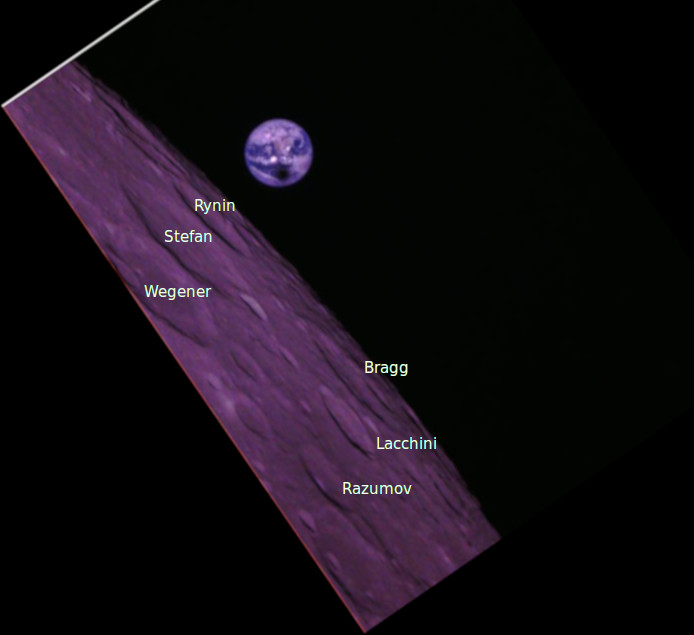
The craters are labelled in the figure below. Important craters in the Coulomb-Sarton basin such as Stefan and Bragg are visible. An image of this region with the craters labelled can be seen here.
I have devoted the lastfewpoststo the planning of the imaging times for the eclipse test run and the validation of the test run done on June 30. This post is a detailed account of the results of the eclipse imaging. Between July 3 and 5, five of the six eclipse images taken on July 2 were downloaded, as well as some other images taken later. Here I give a summary of the downloads during these days and compare the images to the predictions I made.
Yesterday I did an analysis of the image taken and downloaded during the test run for the imaging of the solar eclipse shadow on the Earth with DSLWP-B on July 2. Only one of the six images taken to validate the camera exposure and pointing and orbit errors was downloaded yesterday. The window to download the remaining images was during today’s activation of the Amateur payload between 05:30 and 07:30 UTC.
Three images were downloaded today, with a few missing chunks. Moreover, Wei Mingchuan BG2BHC has sent me better ephemeris, which give a more accurate prediction of the orbit both on the June 30 test run and on the eclipse imaging run on July 2. This post is an analysis of the images downloaded today.
As described in one of my latest posts, today DSLWP-B has made a test imaging run in preparation for the solar eclipse on July 2. A series of images was taken just before the Moon hid the centre of the camera field of view and just after the Moon left the centre of the image, in approximately the same relative positions as for the July 2 eclipse imaging run.
The activation of the Amateur payload started at 05:30 UTC and the payload was commanded to change the configuration of the camera to use 2x zoom. The satellite was occulted by the Moon at 05:40 UTC, preventing the reception of telemetry until it reappeared at 06:16 UTC. The first series of images was taken automatically between 05:51 and 05:54, with the satellite behind the Moon.
After the satellite reappeared from behind the Moon, telemetry confirmed that three images, with IDs 0xD9, 0xDA and 0xDB had been taken. Between 06:29 and and 06:32, the satellite took the second series of images. Telemetry confirmed that these images were taken correctly with IDs 0xDC, 0xDD and 0xDE.
The priority was to use the rest of the activation to download images 0xDA and 0xDD, taken respectively at 05:52:40 and 06:31:10 UTC (when reading the times given in the planning post, note that the times listed there are the moments when the command is sent to the payload by the satellite, but the payload needs about 20 additional seconds to take the image). However, there were difficulties in commanding the payload, so half an hour was lost trying to command the satellite and only image 0xDA could be downloaded before the payload went off at 07:30 UTC.
Image 0xDA was downloaded without errors in a single transmission. It is shown below.
Image 0xDA, taken on 2019-06-30 05:52:40, downloaded between 07:11 ad 07:26
As we see, the exposure of the image is correct, so this image validates that the camera configuration can be used for the eclipse imaging run. Additionally, the image can be used to evaluate camera pointing and ephemeris errors.
As computed in this Jupyter notebook, the separation between the Moon rim and the centre of the field of view in the image shown above is 6.47 degrees. Using the camera calculations Jupyter notebook that I have shown in previous posts, we see that, according to the 20190630 ephemeris from dslwp_dev and my GMAT calculations, the angular distance between the Moon rim and the centre of the image at 05:52:40 UTC should be 3.25 degrees, assuming that the camera points perfectly away from the Sun.
The rate at which the Moon rim moves through the field of view is approximately 0.029 degrees per second. Thus, if the camera was pointing perfectly away from the Sun, this would indicate that DSLWP-B is 110 seconds earlier in its orbit that what predicted by the ephemeris, so that events concerning the relative position of the satellite and the Moon happen 110 seconds later than predicted.
However, one should take these calculations with a grain of salt. In my astrometry post, I showed that the camera was pointing 3.25 degrees off-axis. Therefore, it is convenient to assume an error of +/-3.25 degrees in the angle measurement done with the image. In units of time, this is +/-111 seconds.
So the data seems to suggest that DSLWP-B is one or two minutes earlier in its orbit and that the imaging times should be compensated by making them one or two minutes later, but there is not enough statistical evidence to support this argument. It will be very interesting to see image 0xDD, which will be downloaded tomorrow. The analysis of this image will give additional data.
In any case, so far it seems that orbit and pointing errors are within the tolerance given by the series of three images, which are taken at -1, 0, and +1 minutes offset from the nominal imaging time computed by Wei.


