DSLWP-B upcoming observations of Moon and Earth

Yesterday I looked at the photo planning for DSLWP-B, studying the appropriate times to take images with the DSLWP-B Inory eye camera so that there is a chance of getting images of the Moon or Earth. As I remarked, the Earth will be in view of the camera over the next few days, so this is a good time to plan and take images.

I asked Wei Mingchuan BG2BHC to compare his calculations with mine and shortly after this he emailed me his planning for observations between October 8 and 10. After measuring the field of view of the camera as 37×28 degrees, we can plot the angular distances between the Moon or Earth and the centre of the camera to check if the celestial body will be in the field of view of the camera.

The image below shows the angular distance between these celestial bodies and the centre of the camera. As we did in the photo planning post, we assume that the camera points precisely away from the Sun. Since the Moon and Earth (especially the Moon) have an angular size of several degrees, we plot the centre of these objects with a dashed line and the edges which are nearest and furthest from the camera centre with a solid line.

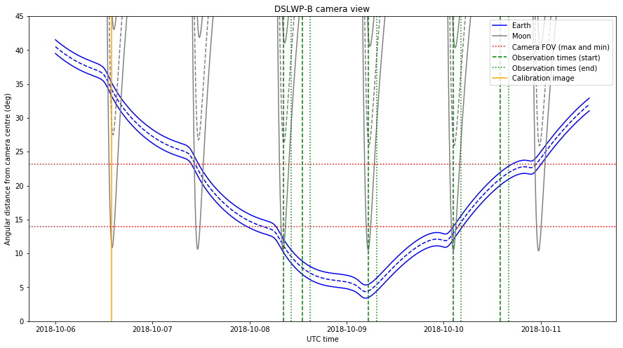
The field of view of the camera is represented with dotted red lines. Since the field of view is a rectangle, we have one mark for the minimum field of view, which is attained between the centre of the image and the centre of the top or bottom edge, and another mark for the maximum field of view, which is attained between the centre of the image and each of the corners.

The rotation of the spacecraft around the camera axis is not controlled precisely, so objects between the two red lines may or may not appear in the image depending on the rotation. Objects below the lower red line are guaranteed to appear if the pointing of the camera is correct and objects above the upper red line will not appear in the image, regardless of the rotation around the camera axis.

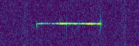
To calibrate the exposure of the camera, an image was taken yesterday on 2018-10-06 13:55 UTC. This time is marked in the figure above with an orange line. The image was downloaded this UTC morning. The download was commanded by Reinhard Kuehn DK5LA and received by Cees Bassa and the rest of the PI9CAM team in Dwingeloo. This image is shown below.

Calibration image taken on 2018-10-06 13:55 UTC

The image shows an over exposed Moon. Here we are interested in using the image to confirm the orientation of the camera. The distance between the centre of the image and the edge of the Moon is 240 pixels, which amounts to 14 degrees. The plot above gives a distance of 11 degrees between the edge of the Moon and the camera centre.

Thus, it seems that the camera is pointed off-axis by 3 degrees. This error is not important for scheduling camera photos, since an offset of a few degrees represents a small fraction of the total field of view and the largest error in predicting what will appear in the image is due to rotation of the spacecraft around the camera axis.

The observations planned by Wei for the upcoming days are shown in the plot above by green lines. The start of the observation is marked with a dashed line and the end of the observation (which is 2 hours later) is marked with a dotted line. The camera should take an image at the beginning of the observation and then we have 2 hours to download the image during the rest of the observation.

We see that Wei has taken care to schedule observations exactly on the next three times that the Moon will be closest to the camera centre. This gives the best chance of getting good images of the lunar surface (but the Moon will only fill the image partially, as in the picture shown above).

There are also two additional observations planned when the Moon is not in view. The first, on October 8 is guaranteed to give a good image of the Earth. The second, on October 10 will only give an image of the Earth if the rotation of the spacecraft is right.

The orbital calculations for the plot shown above have been done in GMAT. I have modified the photo_planning.script script to output a report with the coordinates of the Earth and the Moon in the Sun-pointing frame of reference (see the photo planning post).

The angle between the centre of the camera and the centre of the Earth of the Moon can be calculated as\[\arccos\left(\frac{x}{\sqrt{x^2+y^2+z^2}}\right),\]where \((x,y,z)\) are the coordinates of the celestial body in the Sun-pointing frame of reference. The apparent angular radius of the celestial body can be computed as\[\arcsin\left(\frac{r}{\sqrt{x^2+y^2+z^2}}\right),\]where \(r\) is the mean radius of the body.

These calculations and the plot have been made in this Jupyter notebook.


DSLWP-B camera field of view

In my previous post, I wondered about what was the field of view of the Inory eye camera in DSLWP-B. Wei Mingchuan BG2BHC has answered me on Twitter that the field of view of the camera is 14×18.5 degrees. However, he wasn’t clear about whether these figures are measured from the centre of the image to one side or between two opposite sides of the image. I guess that these values are measured from the centre to one side, since otherwise the total field of view of the camera seems too small.

Here I measure the field of view of the camera using the image of Mars and Capricornus taken on August 4, confirming that these numbers are measured from the centre of the image to one side, so the total field of view is 28×37 degrees.

DSLWP-B clock running late

This Wednesday, a DSLWP-B test was done between 04:00 and 06:00 UTC. During this test, a few stations reported on Twitter that they were able to receive the JT4G signal correctly (they saw the tones on the waterfall) but decoding failed.

It turns out that the cause of the decoding failures is that the DSLWP-B clock is running a few seconds late. Thus, the JT4G transmission starts several seconds after the start of the UTC minute and so the decoding fails, since WSJT-X only searchs for a time offset of a few seconds.

Lunar orbit perturbations and DSLWP-B

Ever since simulating DSLWP-B’s long term orbit with GMAT, I wanted to understand the cause of the periodic perturbations that occur in some Keplerian elements such as the eccentricity. As a reminder from that post, the eccentricity of DSLWP-B’s orbit shows two periodic perturbations (see the figure below). One of them has a period of half a sidereal lunar month, so it should be possible to explain this effect from the rotation of the Moon around the Earth. The other has a period on the order of 8 or 9 months, so explaining this could be more difficult.

DSLWP-B eccentricity

In this post I look at how to model the perturbations of the orbit of a satellite in lunar orbit, explaining the behaviour of the long term orbit of DSLWP-B.

Aircraft reflections of a 2.3GHz beacon

A couple months ago, Andrés Calleja EB4FJV installed a 2.3GHz beacon in his home in Colmenar Viejo, Madrid. The beacon has 2W of power, radiates with an omnidirectional antenna in the vertical polarization, and transmits a tone and CW identification at the frequency 2320.865MHz.

Since Colmenar Viejo is only 10km away from Tres Cantos, where I live, I can receive the beacon with a very strong signal from home. The Madrid-Barajas airport is also quite near (15km to the threshold of runway 18R) and several departure and approach aircraft routes pass nearby, particularly those flying over the Colmenar VOR. Therefore, it is quite easy to see reflections off aircraft when listening to the beacon.

On July 8 I did a recording of the beacon from 10:04 to 11:03 UTC from the countryside just outside Tres Cantos. In this post I will examine the aircraft reflections seen in the recording and match them with ADS-B aircraft position and velocity data obtained from adsbexchange.com. This will show the locations and trajectories which produce reflections strong enough to be detected.

Amateur stations in the Perseids recording

In one of my latest posts I analysed the meteor scatter pings from GRAVES on a recording I did on August 11 (see that post for more details about the recording). The recording covered the frequency range from 142.5MHz to 146.5MHz and was 1 hour and 34 minutes long. Here I look at the Amateur stations that can be heard in the recording. Note that Amateur activity in meteor scatter communications increases considerably during large meteor showers, due to the higher probabilities of making contacts.

Detecting meteor scatter pings from GRAVES during the Perseids

GRAVES is a French space surveillance radar that transmits with very high power at 143.050MHz. It is easy to receive it from neighbouring countries via meteor scatter. During this year’s Perseids meteor shower I did a recording of GRAVES and the 2m Amateur band for later analysis. The recording was done at 08:56 UTC of Saturday 12th August and it is about 1 hour and 34 minutes long. Here I present an algorithm to detect and extract the meteor scatter pings from GRAVES.

Report for today’s DSLWP-B SSDV session

Today an SSDV transmission session from DSLWP-B was programmed between 7:00 and 9:00 UTC. The main receiving groundstation was the Dwingeloo radiotelescope. Cees Bassa retransmitted the reception progress live on Twitter. Since the start of the recording, it seemed that some of the SSDV packets were being lost. As Dwingeloo gets a very high SNR and essentially no bit errors, any lost packets indicate a problem either with the transmitter at DSLWP-B or with the receiving software at Dwingeloo.

My analysis of last week’s SSDV transmissions spotted some problems in the transmitter. Namely, some packets were being cut short. Therefore, I have been closely watching out the live reports from Cees Bassa and Wei Mingchuan BG2BHC and then spent most of the day analysing in detail the recordings done at Dwingeloo, which have been already published here. This is my report.

DSLWP-B corrupted SSDV frames

In my previous post I looked at the first SSDV transmission made by DSLWP-B from lunar orbit. There I used the recording made at the Dwingeloo radiotelescope and showed how to decode the SSDV frames and produce a JPEG image.

Only four SSDV frames where transmitted by DSLWP-B, and out of those four, only two could be decoded correctly. I wondered why the decoding of the other two frames failed, since the SNR of the signal as recorded at Dwingeloo was very good, yielding essentially no bit errors (even before FEC decoding).

Now I have looked at the signal more in detail and have found the cause of the corrupted SSDV frames. I have demodulated the signal in Python and have looked at the position where an ASM (attached sync marker) is transmitted. As explained in this post, the ASM marks the beginning of each Turbo codeword. The Turbo codewords are 3576 symbols long and contain a single SSDV frame.

A total of four ASMs are found in the GMSK transmission that contains the SSDV frames, which matches the four SSDV transmitted. However, the distance between some of the ASMs doesn’t agree with the expected length of the Turbo codeword. Two of the Turbo codewords where cut short and not transmitted completely. This explains why the decoding of the corresponding SSDV frames fails.

The detailed analysis can be seen in this Jupyter notebook.

This is rather interesting, as it seems that DSLWP-B had some problem when transmitting the SSDV frames. I have no idea about the cause of the problem, however. It would be convenient to monitor carefully future SSDV transmissions to see if any similar problem happens again.

DSLWP-B long-term orbit evolution

In my last post I commented that one of the motivations for the periapsis raise manoeuvre of DSLWP-B on July 20 was to prevent the satellite from crashing into the Moon in a few months. When Wei Mingchuan BG2BHC told me this, I found it a bit surprising, since I had the impression that the periapsis had been raising naturally since the satellite was injected in lunar orbit on May 25. Thus, I decided to propagate the orbit for a period of 2 years using GMAT and study the long-term effects in the Keplerian elements.