Open Research Institute has recently published the solutions for a Lunar Descent CTF that they ran at BSides San Diego 2026. The CTF revolves around the Ka-band radio altimeter used by the Chandrayaan-3 lunar lander. The CTF includes a simulation of the radio altimeter and the goal is to discover why the lander is crashing in this simulation and fix the problem. The CTF is in the Github repository OpenResearchInstitute/lunar-descent-ctf, which includes both the CTF and the solutions (in a spoilers directory). This seemed like an interesting topic, and in the past I have enjoyed a lot other CTFs that were organized by Michelle Thompson, so I decided to clone the repo, delete the spoilers directory, and start playing. In this post I comment on the CTF and my solution, so read no further if you don’t want to see spoilers.
Author: destevez
Tianwen-2 low data rate telemetry
Thomas Telkamp has shared with me an IQ recording of the Tianwen-2 telemetry downlink made with the Bochum 20 metre antenna on June 8. This is part of an ongoing effort led by Peter Gülzow, AMSAT-DL‘s president, for closely monitoring Tianwen-2’s operations. All the material I have used in previous posts about Tianwen-2 has come from these activities.
This recording was made just before Tianwen-2 did a manoeuvre (recall that the orbital insertion at asteroid Kamo’oalewa was reported to be on June 7). During this recording Tianwen-2 was transmitting telemetry at a slower rate than the usual 16384 baud. This makes sense, given the fact that the attitude during the manoeuvre would be unfavourable. In this short post I decode this recording.
The only two configuration differences between the regular 16 kbaud telemetry and this lower data rate telemetry is that the baudrate is reduced to 4096 baud, and the frame size is reduced to 220 bytes. This means that a single Reed-Solomon codeword from the shortened (252, 220) code is used, instead of four interleaved Reed-Solomon codewords from the full (255, 223) code. The over-the-air frame duration is still one second.
The corresponding modifications to the GNU Radio decoder are simple. This plot shows the decoder running on the recording. The SNR is excellent.
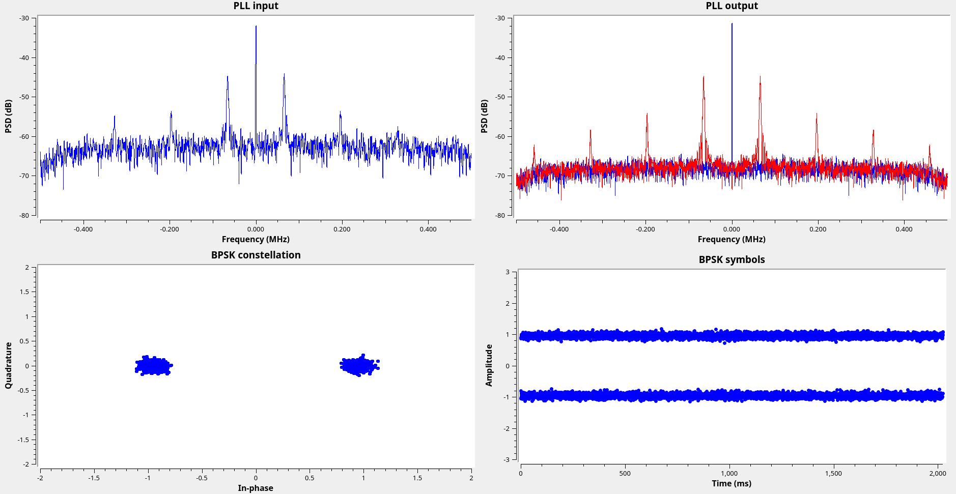
The contents of the telemetry frames are the same as the regular 16384 baud telemetry. There are very few differences. One difference is that the last two bytes of the AOS insert zone, which are always 0x300b in 16384 baud telemetry, are always 0x0001 in this 4096 baud telemetry. I don’t know what these bytes mean, and this difference doesn’t give me a clue either.
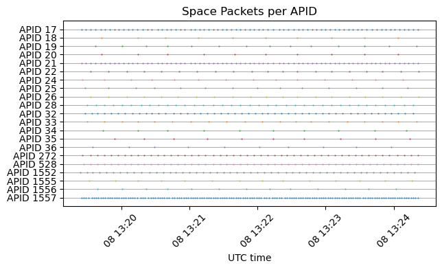
Almost all the same APIDs as in the regular telemetry are present, although their transmission rate is reduced due to the lower data rate. Comparing, I see that only APIDs 1553 and 1554 are missing in the low rate telemetry.
The GNU Radio decoder used in this post is here, the Jupyter notebook is here, and the binary file containing the decoded frames is here.
PLL coefficients for rate-only feedback
A couple years ago I wrote a post about the paper Controlled-Root Formulation for Digital Phase-Locked Loops, by Stephens and Thomas. In this paper, the authors study digital PLLs by studying the transfer function in discrete time, rather than doing any continuous-time approximations or equivalences. They give values for the loop coefficients that are needed to achieve a certain noise bandwidth for some standard loop root placements (the supercritical damped response and the standard underdamped response). In general, the loop coefficients are obtained numerically. In my post, I show that in the case of a loop of order 2 with supercritical response the loop coefficients can be calculated explicitly in terms of the loop bandwidth by using the solution of a cubic equation. However, in that post, I treated only the phase/phase-rate feedback case. In this post I cover the rate-only feedback case.
An update about Tianwen-2 telemetry
Yesterday I posted about my decoding of some recordings of the X-band telemetry of Tianwen-2 done by the Dwingeloo radio telescope. Today I have some small updates.
First of all, I have figured out the format of the AOS insert zone. In the previous post I mentioned that the AOS insert zone contains 8 bytes that are mostly static, except for one byte that seems to be a frame counter. I suspected that the AOS insert zone would contain timestamps, which was the case with Tianwen-1, but this didn’t seem to be the case with Tianwen-2. However, today I have found that the 8-byte insert zone contains a 6-byte timestamp in little endian format that counts the number of \(2^{-16}\) second ticks since the epoch, which is 2019-12-31 16:00:00 UTC (or 2020-01-01 00:00:00 Beijing time). The remaining two bytes have the constant value 0x300b. I don’t know what these two bytes are, since they don’t seem to be a CCSDS time code P-field.
There were two things about this timestamp field that were confusing me: the fact that it is little-endian, since CCSDS and the telemetry data in the Space Packet payloads is always big-endian, and the fact that these AOS frames take exactly one second to transmit. This means that the change in the timestamp in each frame is just an increment in the byte corresponding to seconds, which carries over to the next bytes on overflows, plus a very slow drift in the least significant byte caused by the relative drift of the symbol rate clock and the spacecraft clock. Only now that I’ve seen how this field evolves during longer periods of time, I have been able to figure its format.
Using an epoch in Beijing time instead of UTC is common in Chinese spacecraft. For instance, Tianwen-1 uses 2016-01-01 00:00:00 Beijing time as its epoch.
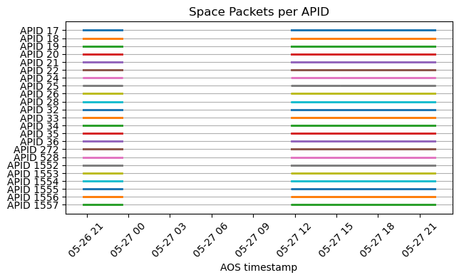
The second update is that AMSAT-DL has been tracking Tianwen-2 with their 20 m dish in Bochum and decoding the telemetry signal in real time with SatDump. They have shared the decoded AOS frames with me, and I have run them through my Jupyter notebook. They have collected a good amount of data: a few hours on May 26 and a full track of about 10 hours on May 27. This data is what has given me the clues to figure out how the timestamps work. The following plot shows the APIDs received over time. This indicates that there are no APIDs that are only active occasionally.
Even though now we have a much longer time span of data, the qualitative behaviour of the telemetry is still the same as I mentioned in the last post. The Jupyter notebook where I analyse the frames received by Bochum is here.
Decoding Tianwen-2
Tianwen-2 is a Chinese mission that will return samples from the Earth quasi-satellite asteroid 469219 Kamoʻoalewa and rendezvous with the 311P/PanSTARRS comet. It was launched on 28 May 2025 from the Xichang Satellite Launch Center. It is planned to perform its orbital insertion at Kamoʻoalewa on 7 June 2026, and study the asteroid until 24 April 2027. Since ephemerides for this mission are not publicly available, it has been difficult for amateur observers to track it so far, but now it is close enough to Kamoʻoalewa to find it by pointing around the asteroid.
On Monday, CAMRAS used the 25 meter Dwingeloo radio telescope to receive and record the X-band telemetry signal from Tianwen-2, publishing the SigMF recordings in their data archive. They reported that the spacecraft was 1.1 degrees away from the asteroid. In this post I will decode and analyse the telemetry using these recordings.
Getting peak TOPS on a Ryzen AI 7 350 NPU
I have a Framework Laptop 13 that has a Ryzen AI 7 350 CPU that includes an NPU. I have started playing with this NPU to understand how to develop software for it. While NPUs are mainly intended as accelerators for inference of ML models, they are fundamentally hardware accelerators for matrix multiplication and other similar linear algebra operations, so they are also useful for signal processing and other compute applications, which is why I am interested in them. Another reason why I am interested in this NPU is that, as I will explain below, it is very similar to the AIE-ML v2 AI engine in Versal FPGA SoCs, so this laptop is a great platform to learn how to use this AI engine.
NPUs use the concept of TOPS (tera operations per second) as a high-level marketing figure of their capabilities. An operation is generally understood as an addition or multiplication for int8 data types, since the amount of parallelization that can be achieved depends on the datatype width. The NPU on the Ryzen AI 7 350 is marketed as a 50 TOPS NPU. The main goal of this post is to understand where this number comes from, in terms of hardware execution units and capabilities, understand under which conditions it can be reached, and write a small application that reaches this TOPS value.
I think this is a good way of gaining in-depth understanding about a compute architecture. Most typical real world use cases are going to be slower than this, because the algorithms will have bottlenecks that result in hardware underutilization. By understanding how the hardware needs to be used to reach peak performance, we have a better idea of the gaps of these algorithms and also how to rewrite the algorithms to reduce the gap if possible. In a post last year about NEON kernels on the ARM Cortex-A53 I worked in a similar way, by choosing a simple kernel to accelerate and by comparing performance benchmarks with the peak performance allowed by the hardware.
Decoding the NB-IoT downlink
Recently I have been posting about V16 beacons, which are car emergency warning beacons that have been introduced this year in Spain, and which use the LTE NB-IoT cellular network to transmit their geolocation data to the traffic authority network when they are switched on. As part of experimenting with these beacons, I made recording of the downlink and uplink NB-IoT signals while the beacon was sending data to the network. My hope was to be able to decode these signals and extract the two-way traffic that shows how the beacon attaches to the LTE network and sends its data. I already decoded all the uplink transmission in a previous post. In this post I will decode the corresponding recording of the downlink channel.
However, as I already suspected when I was decoding the uplink recording, due to how I physically set up the experiment to avoid saturating the SDR receiver with the beacon transmissions, it turns out that the beacon was talking to an NB-IoT cell that is relatively weak in the downlink recording. More specifically, the antenna for the SDR receiver was set up near a window in the north side of the house, while the beacon was placed on the window sill on the south side of the house. The SDR receiver sees strong downlink signals from cell 145, which is located northeast of the house and is the cell to which the beacon connected in a previous experiment I did with the beacon placed in the north window. However, in this experiment with the beacon on the south window, the beacon connected to cell 261, which is southwest of the house. The signal from this cell is weaker in the downlink recording and is frequently overwhelmed by the signals from cell 145 and other strong cells. So I have had partial success decoding the transmissions that the network sent to the beacon.
This post is mainly about the NB-IoT downlink in general. At the end I focus on the downlink transmissions to the V16 beacon that I have been able to decode. It is a rather long post, because I cover all the main physical channels and signals of the NB-IoT downlink. I show how the NPSS and NSSS primary and secondary synchronization signals and the NRS reference signals work, how to decode the MIB-NB in the NPBCH, how to decode the SIB1-NB and SI messages carrying other SIB-NBs, how to decode NPDCCH transmissions in the Type1 common search space, which corresponds to paging, as well as decoding the corresponding NPDSCH transmissions carrying paging messages, how to do blind decoding of NPDCCH transmissions in the Type2 common search space and UE-specific search space, which correspond to uplink grants and downlink scheduling, and decode the corresponding NPDSCH transmissions that send data to the V16 beacon.
The recording used in this post is published in the dataset Recording of the NB-IoT downlink of a V16 beacon in Zenodo.
Tianwen-1 received again by AMSAT-DL
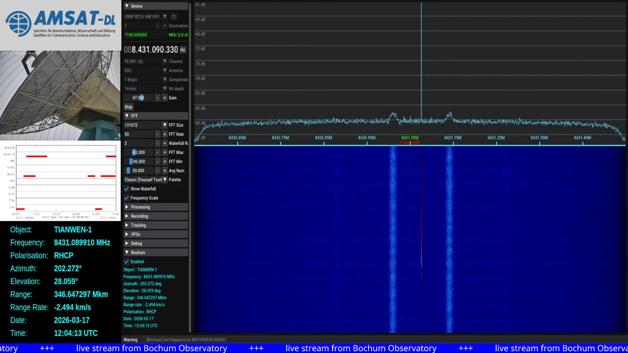
A few days ago I posted about the fact that AMSAT-DL had not received any signals from Tianwen-1 since 2025-12-23. For months, AMSAT-DL had kept listening to the orbiter’s frequency with the 20 m antenna in Bochum and had not detected any signals. Yesterday, AMSAT-DL announced that they had received again the signal from Tianwen-1.
The signal strength looks completely normal, as evidenced by the spectrum plot shared in the announcement.
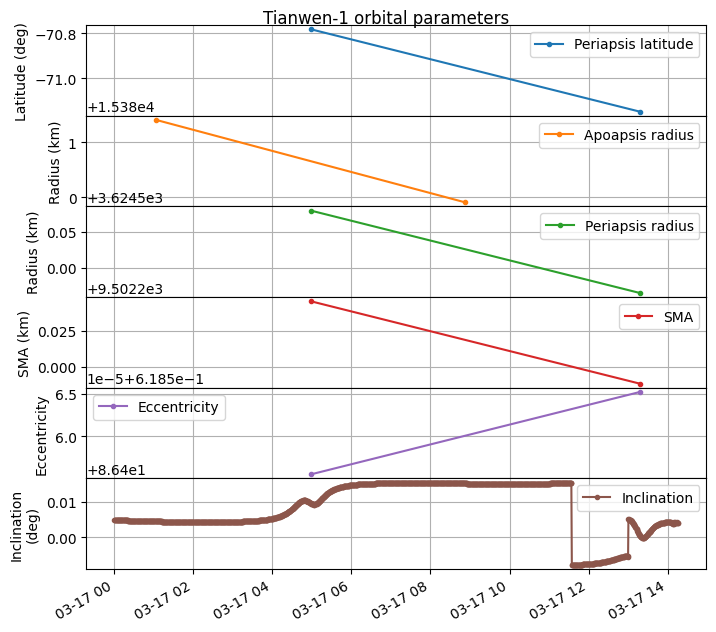
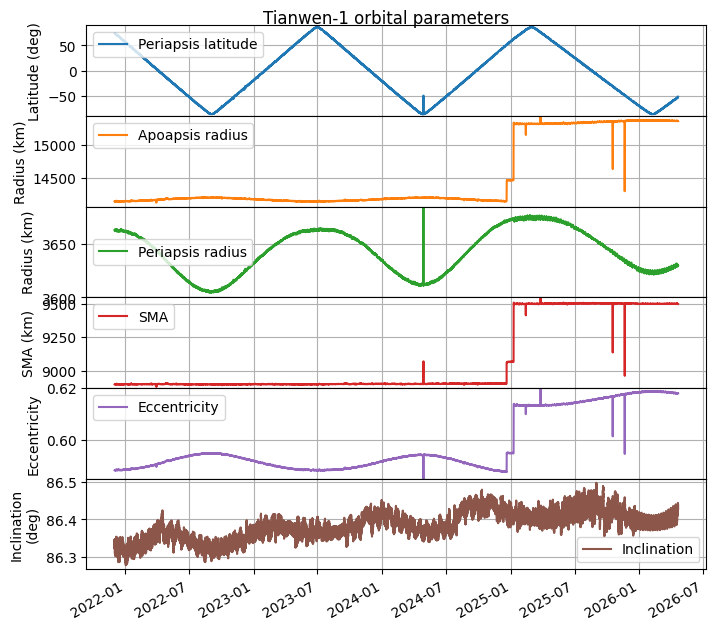
Telemetry containing state vectors was decoded between 2026-03-17 11:34 and 14:16 UTC. I have updated my plot of orbital parameters to include this new information. The period between 2025-12-23 and 2026-03-17 corresponds to a propagation with GMAT of the last telemetry received in 2025. The end of the plot corresponds to the telemetry received in 2026-03-17.
We can see that the orbit has remained the same, and there have been no manoeuvres during this period. A zoomed in version to the end of the plot shows that there is basically no jump in the orbital parameters. There is a tiny jump in the inclination as the new telemetry is received, but that is all.
So far the reasons why Tianwen-1 has apparently not transmitted telemetry to Earth for almost 3 months remain unknown.
Where is Tianwen-1?
Yesterday, AMSAT-DL published the news that they have been unable to receive any signals from Tianwen-1 with the 20 m antenna in Bochum since 2025-12-23. As you may know if you have been following my posts about Tianwen-1, AMSAT-DL has been using this antenna to receive and decode telemetry from Tianwen-1 almost every day since the beginning of the mission in 2020-07-23. The news about the lack of signal detected from Tianwen-1 over the last few months were hardly a secret, because AMSAT-DL runs a livestream of the signals received with the Bochum antenna 24/7, so anyone could look at the livestream and realize that Tianwen-1 was being observed but no signal was visible on the spectrum. However, now that the public has been made well aware of this fact, I can make some more comments about it. There has been no public communication from the Chinese space program regarding this, so the fate of Tianwen-1 is currently unknown.
During December 2025 and January 2026, there was a Mars conjunction, which means that Mars goes behind the Sun as seen from Earth. Communications with Mars orbiters cannot happen during this period of time. For instance, this news piece hints at NASA Mars missions not having contact between 2025-12-29 and 2026-01-16, which corresponds to a Sun-Earth-Mars angle (elongation) of 3º on 2025-12-29 and 1.8º on 2026-01-16, with the minimum elongation achieved on 2026-01-09. Therefore, it was completely expected that we would lose Tianwen-1’s signal during the conjunction period. Because the communications link to Earth does not work, spacecraft will usually not point their high gain antennas to Earth and even stop transmitting during this period. However, we expected to see Tianwen-1 back again after the conjunction, and we never did.
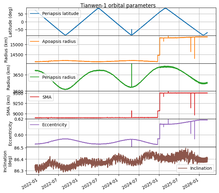
I have been using the telemetry decoded by AMSAT-DL, which includes the spacecraft state vectors, to keep track of the spacecraft orbit. I have been posting updates about any change that happens. The last one was the apoapsis raise on 2025-01-08. The lack of signals from Tianwen-1 sparked internal discussion about whether the spacecraft might have intentionally reentered some time around the conjunction period as a way of terminating the mission without leaving orbital debris. To analyse whether this could be possible, I have updated my orbit analysis to account for all the telemetry that has been received so far, up to 2025-12-22, which is when the last telemetry was decoded.
The result can be seen in the figure below. We see the apoapsis raises that happened during the end of 2024 and beginning of 2025. After that there have been no manoeuvres.
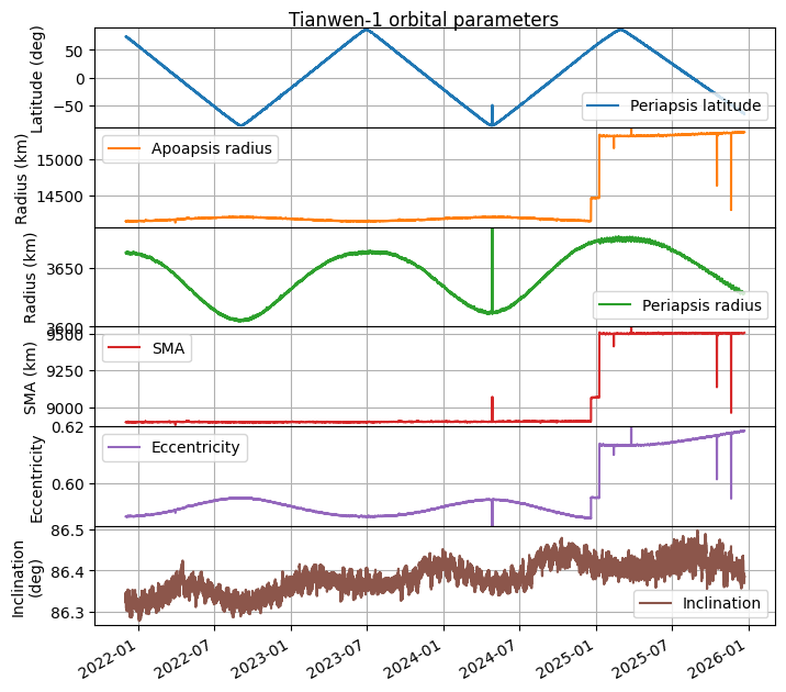
Since the plot above indicates that the periapsis radius would be going towards a minimum at the beginning of 2026 due to long-term periodic orbit perturbations, I propagated the last telemetry data we have forward with the goal of studying the impact of the larger apoapsis radius. The results are shown here. We note that the apoapsis radius minimum is now much higher than in the past, so the hypothesis of a reentry is unlikely unless a manoeuvre that we didn’t see in the telemetry has happened.
I have update the Jupyter notebook that has made these plots.
ESCAPADE telemetry
Back in November, I posted about the ESCAPADE Mars twin orbiter mission. I made a recording of the X-band telemetry with the Allen Telescope Array the day after launch, and I decoded the telemetry with GNU Radio. I made a preliminary analysis of the telemetry, showing that it contained a large number of log messages in ASCII. Shortly after writing this post, PistonMiner provided a deeper analysis of the telemetry, including a Github repository with some code and extracted data. She noticed that the CCSDS Space Packets, all of which belonged to the same APID 51, contained MAX simple telemetry frames in their payloads. Since MAX telemetry frames contain their own APIDs, this allowed separating the different types of telemetry data. Since seeing this, I wanted to go back and analyse again the telemetry to see what else I could find. Now I’ve finally had some time to do this. In this post I describe my new findings, as well as what PistonMiner originally discovered.