Coherence and QO-100

My tweet about the AMSAT-BR QO-100 FT8 QRPp experiment has spawned a very interesting discussion with Phil Karn KA9Q, Marcus Müller and others about weak signal modes specifically designed for the QO-100 communications channel, which is AWGN albeit with some frequency drift (mainly due to the imperfect reference clocks used in the typical groundstations).

Roughly speaking, the conversation shifted from noting that FT8 is not so efficient in terms of EbN0 to the idea of using something like coherent BPSK with \(r=1/6\) CCSDS Turbo code, then to observing that maybe there was not enough SNR for a Costas loop to work, so a residual carrier should be used, and eventually to asking whether a residual carrier would work at all.

There are several different problems that can be framed in this context. For me, the most interesting and difficult one is how to transmit some data with the least CN0 possible. In an ideal world, you can always manage to transmit a weaker signal just by transmitting slower (thus maintaining the Eb/N0 constant). In the real world, however, there are some time-varying physical parameters of the signal that the receiver needs to track (be it phase, frequency, clock synchronization, etc.). In order to detect and track these parameters, some minimum signal power is needed at the receiver.

This means that, in practice, depending on the physical channel in question, there is a lower CN0 limit at which communication on that channel can be achieved. In many situations, designing a system that tries to approach to that limit is a hard and interesting question.

Another problem that can be posed is how to transmit some data with the least Eb/N0 possible, thus approaching the Shannon capacity of the channel. However, the people doing DVB-S2 over the wideband transponder are not doing it so bad at all in this respect. Indeed, by transmitting faster (and increasing power, to keep the Eb/N0 reasonable), the frequency drift problems become completely manageable.

In any case, if we’re going to discuss about these questions, it is important to characterize the typical frequency drift of signals through the QO-100 transponder. This post contains some brief experiments about this.

To measure the typical frequency drift on the QO-100 transponder, I have decided to record the lower CW beacon of the NB transponder using my groundstation. The beacon is transmitted at Bochum using a very stable Z3801A GPSDO as a reference. My station is currently using the DF9NP GPSDO that I measured here. This GPSDO is a VCTCXO disciplined by a uBlox GPS receiver, so its short-time performance is typical of a TCXO.

I reckon that results perhaps an order of magnitude better might be obtained with a good OCXO-based GPSDO, such as the Vectron I used here, but I wouldn’t like to devise a communications system that requires an extremely stable clock. Certainly, FT8 and other modes work well with the DF9NP GPSDO, so I think it’s best to use it instead of the Vectron for this experiment.

The CW beacon transmits a continuous carrier with a duration of 12 seconds after each message. I have made a short recording of the beacon that includes three of these carriers. The recording can be downloaded here at 1ksps in complex64 format. The figure below shows a waterfall of the recording in inspectrum. The frequency “wiggle” is approximately 10Hz.

Coherence time

I have selected 11 seconds of each of the occurrences of the carrier and processed them in this Jupyter notebook to measure the coherence time. The technique I have used is based on the following method for finding the coherence time of a carrier at baseband. If \(\{x_k\}\), \(0 \leq k < L\) is the discrete time baseband complex-valued representation of that carrier, for each decomposition \(L = MN\) we define\[P_N = \frac{1}{M}\sum_{l = 0}^{M-1} \left|\frac{1}{N}\sum_{k=0}^N x_{Nl + k}\right|^2\]as the average power after coherent accumulations of \(N\) samples are done. By plotting \(P_N\) we can find a point at which \(P_N\) starts decreasing with increasing \(N\). This indicates the time length at which coherence is lost.

Since the CW carrier is not at baseband in this recording, but rather at a frequency around -50Hz, I first detect the average frequency of each carrier using an FFT and then shift the carrier down to baseband using that frequency. The figure below shows the coherence time, as described above. Each of the traces represents one of the three carriers. The green one is the last one, which is clearly seen to drift more in the waterfall.

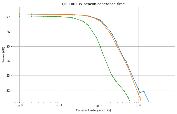
A serious version of this experiment would use a much longer recording and average the results over many occurrences of the 12 second carrier, rather than examining only three occurrences. However, for a ballpark estimate I think this is enough and we may say that the coherence time for a typical TCXO-based station is on the order of 50 to 100ms.

PLL lock

The second part of the experiment is to try to lock a PLL on the carrier at different levels of CN0. The carrier has been recorded with a high CN0, so lower values of CN0 can be simulated by adding white Gaussian noise. I have selected the last occurrence of carrier, as it is the worst one, and play it in a continuous loop in GNU Radio using this flowgraph. Interestingly, the phase and frequency discontinuity at the looping point doesn’t seem to give any problems with the PLL.

I have scaled the signal so that the carrier has amplitude one. This makes it easy to add noise to set the desired CN0. The signal is lowpass filtered to an adjustable bandwidth and locked with a PLL of adjustable bandwidth.

To aid in examining the performance of the PLL, I use a noise-free version of the signal and use the phase of the PLL running on the noisy signal to lock the noise-free signal. This shows the PLL jitter very well.

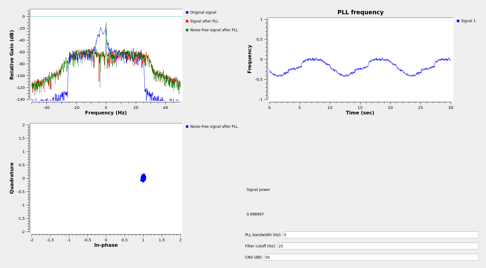
The PLL simulation can be seen in the figure below. For a high CN0 and relatively high PLL bandwidth of 5Hz, the PLL jitter (as seen on the noise-free signal) is low. The original signal (in blue in the frequency plot) looks spread in frequency, while the output of the PLL is locked.

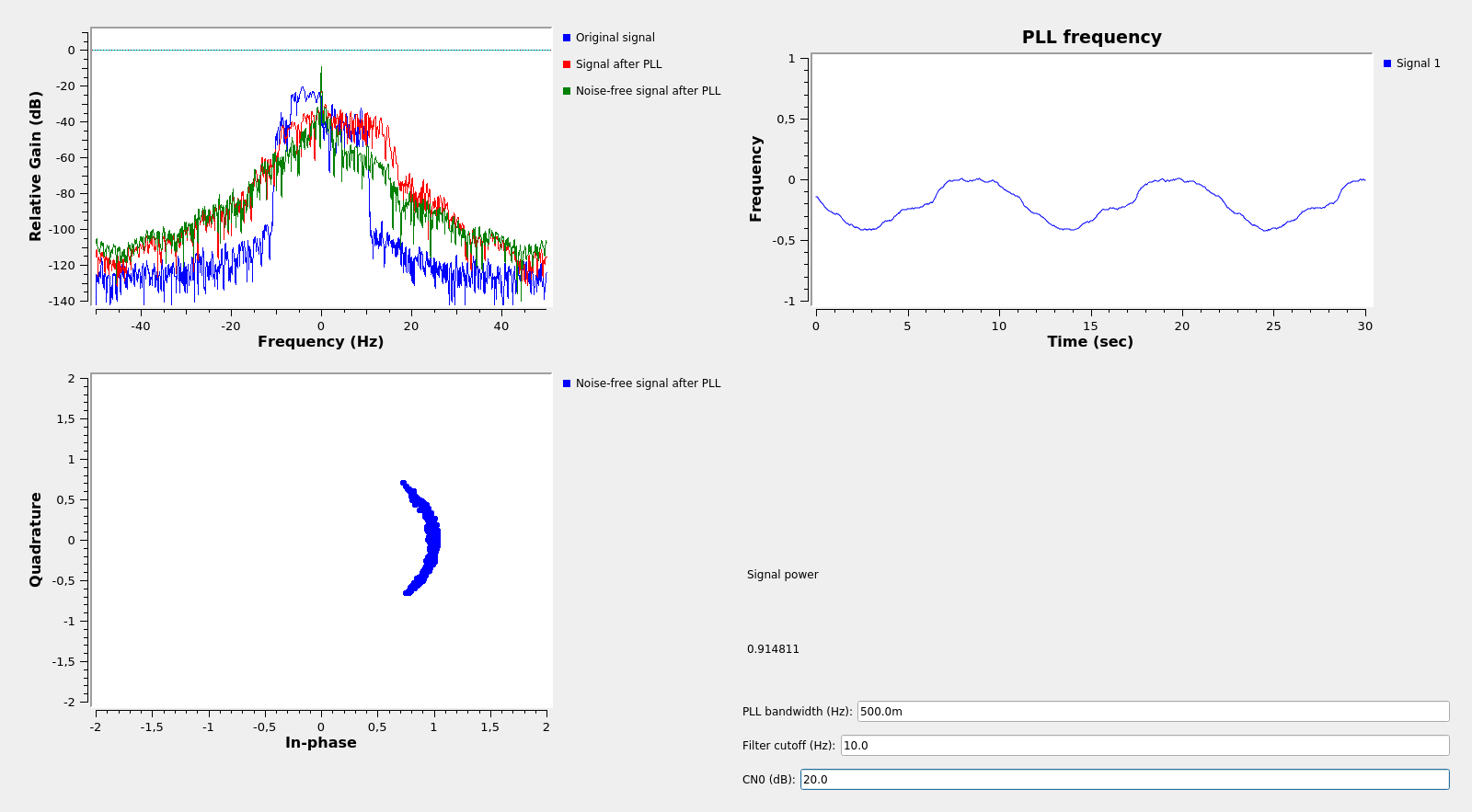
If we reduce the CN0 to 20dB, the PLL jitter is considerable, as it can be seen both on the PLL frequency output and in the constellation of the noise-free signal. To judge the effect of the PLL jitter, I average coherently the noise-free signal (after using the output of the PLL to lock it) and compute its power. In this case it is 0.8, so we’ve lost 20% signal power because of the PLL jitter.

To try to improve things, we can reduce the bandwidth of the lowpass filter to 10Hz (anything lower will cut the signal sometimes, as it drifts outside of the passband) and reduce the PLL bandwidth to 1 or 0.5Hz. This results in the figure below, in which the situation improves and we get a signal power of 0.9.

However, reducing the bandwidth to 0.5Hz is as low as we can get. Indeed, if we increase the CN0 maintaining the bandwidth parameters, we get the figure below, which shows approximately the same PLL jitter. This means that the jitter is not caused by thermal noise due to low SNR, but rather by loop stress due to the low loop bandwidth.

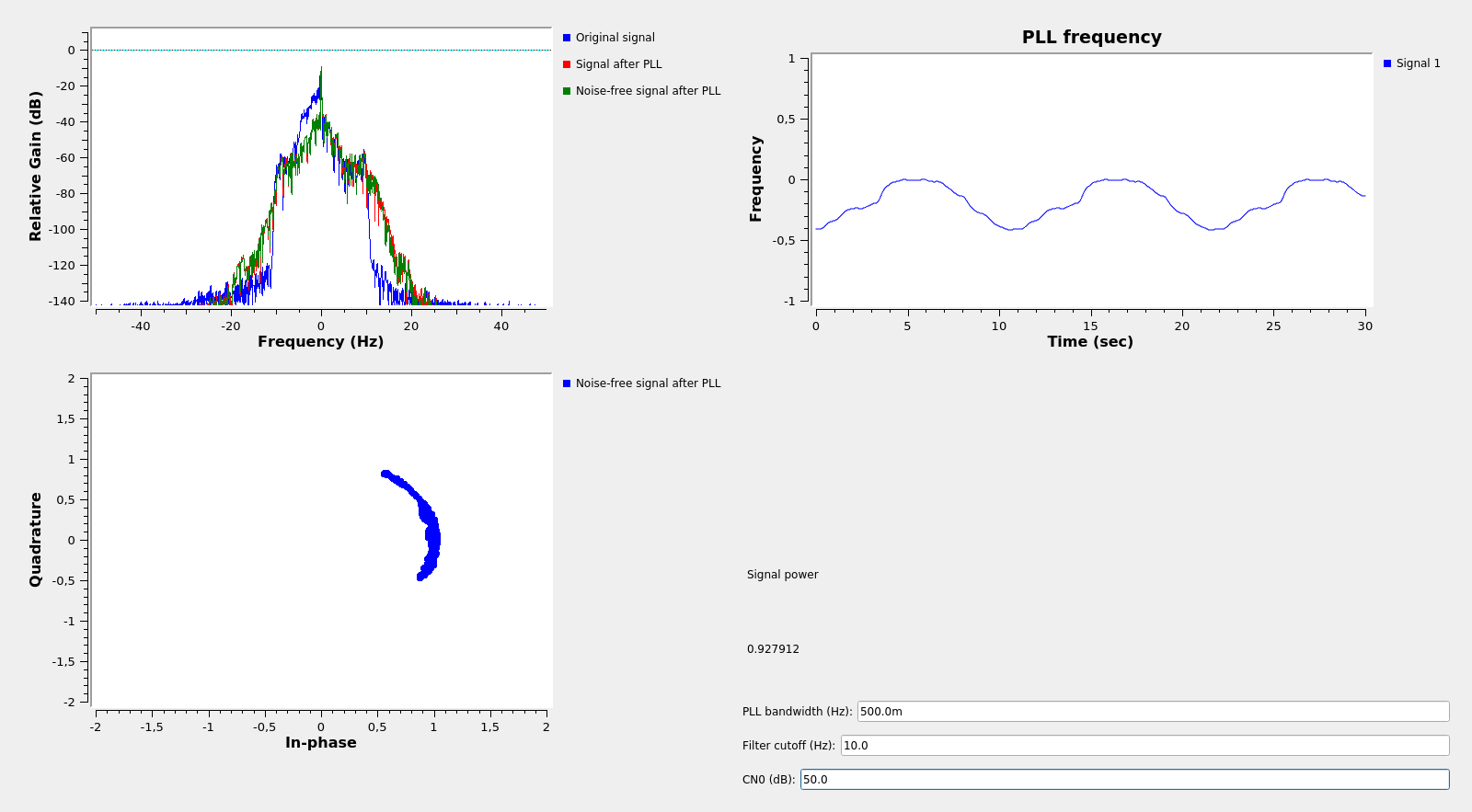
If we keep a high CN0 but reduce the loop bandwidth further to 0.3Hz, we get bad results, as shown below. Reducing the bandwidth further will make the loop lose lock completely.

However, 20dB CN0 is still very high for what we have in mind. To put things into perspective, in the AMSAT-BR experiment we were playing with FT8 signals at -22dB SNR in 2.5kHz. This is a CN0 of 12dB. If we want to do somewhat better than FT8 with a residual carrier signal, we should think of a carrier power of 10dB CN0 or less, as we still need some power for the data.

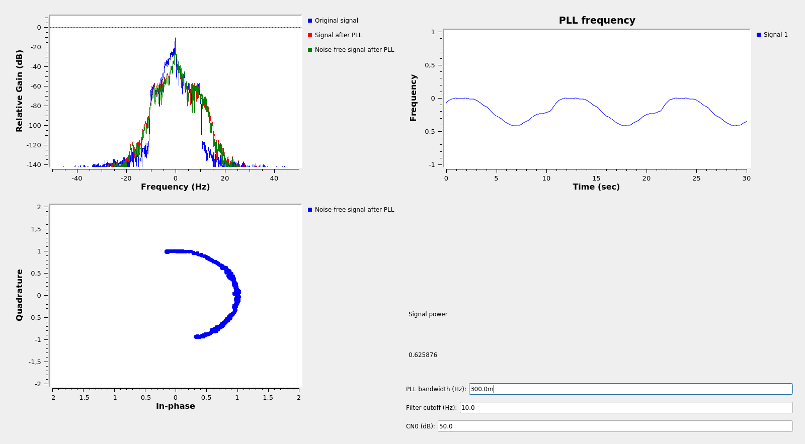
The results at 10dB CN0 with a loop bandwidth of 0.5Hz can be seen below. The loop loses lock sometimes and the jitter is really bad. The signal power is around 0.6. So it seems that this is as far as we can push the system.

Phil Karn mentioned the article Residual Versus Suppressed-Carrier Coherent Communications. This paper contains some useful formulas regarding when to choose a suppressed carrier system or a residual carrier one, what is the optimal power fraction to allocate for the residual carrier, and when can a PLL or Costas loop maintain lock.

The rule for PLL lock is that the loop SNR \(\rho\) should be greater than 7dB, where\[\rho = \frac{C}{N_0 B_L}.\]Here \(B_L\) denotes the Loop bandwidth in Hz. This agrees with my experimental results. For \(B_L = 0.5\mathrm{Hz}\) we have \(\rho = 7\mathrm{dB}\) when CN0 = 10dB.

The challenge

With these results in mind, I think I can justify as rather challenging the idea of trying to transmit data at very low CN0 through the QO-100 transponder. To keep things reasonable and concrete, let’s assume that we want to transmit at more or less the same net bitrate as FT8, which is 7.2 bits per second.

A -22dB in 2.5kHz SNR FT8 signal has an Eb/N0 of 3.4dB. It is perhaps arguable whether the signals estimated by WSJT-X to have -22dB SNR really have that SNR or if the real SNR is somewhat higher. However, in any case, by trying to use a better modulation and FEC, one may try to go down to 1dB Eb/N0, or even less.

A 1dB Eb/N0 signal at 7.2 bits per second has a CN0 of 9.6dB. Now this is the challenge. Clearly a residual carrier approach is not going to work, and suppressed carrier coherent BPSK won’t work either.