Last Sunday, I used Scott Tilley VE7TIL’s Doppler measurements of the DSLWP-B S-band beacon to perform orbit determination using GMAT. Yesterday Scott sent me the Doppler data he has been collecting during this week. I have re-run my orbit determination process to include this new data.
Below I show the Keplerian state that was determined on 2018-06-03, in comparison with the new state determined on 2018-06-10 (both are referenced to the same epoch of 2018-05-26 00:00:00 UTC).
% 20180603
%DSLWP_B.SMA = 8761.0758581
%DSLWP_B.ECC = 0.768016853537
%DSLWP_B.INC = 16.9728174682
%DSLWP_B.RAAN = 295.670653562
%DSLWP_B.AOP = 130.427472407
%DSLWP_B.TA = 178.126596496

% 20180610
DSLWP_B.SMA = 8762.40279943
DSLWP_B.ECC = 0.764697135746
DSLWP_B.INC = 18.6101083906
DSLWP_B.RAAN = 297.248156986
DSLWP_B.AOP = 130.40460851
DSLWP_B.TA = 178.09494681
It seems that there is still an indetermination of a few degrees in the inclination and right-ascension of the ascending node and a few kilometres in the semi-major axis.
The graph below shows the Doppler fit.
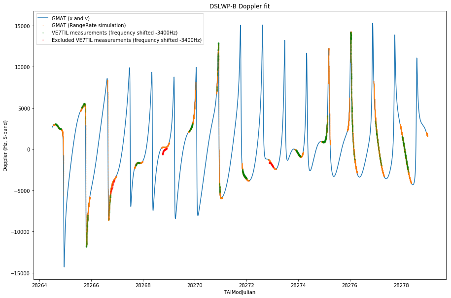
The Jupyter notebook where these calculations are performed can be found here.