In my previous post, I examined a recording of LilacSat-1 transmitting an image. I did some calculations regarding the time it would take to transmit that image and the time that it actually took to transmit, given that the image was interleaved with telemetry packets. I wondered if the downlink KISS stream capacity was being used completely.
You can find more information about the downlink protocol of LilacSat-1 in this post. The important information to know here is that it consists of two interleaved channels: a channel that contains Codec2 frames for the FM/Codec2 repeater and a channel that contains a KISS stream. The KISS stream is sent at 3400bps. At any moment in time, the KISS stream can be either idling, by sending c0 bytes, or transmitting a CSP packet. The CSP packets can be camera packets (which are sent to CSP destination 6) or telemetry packets (and perhaps also other kinds of packets).
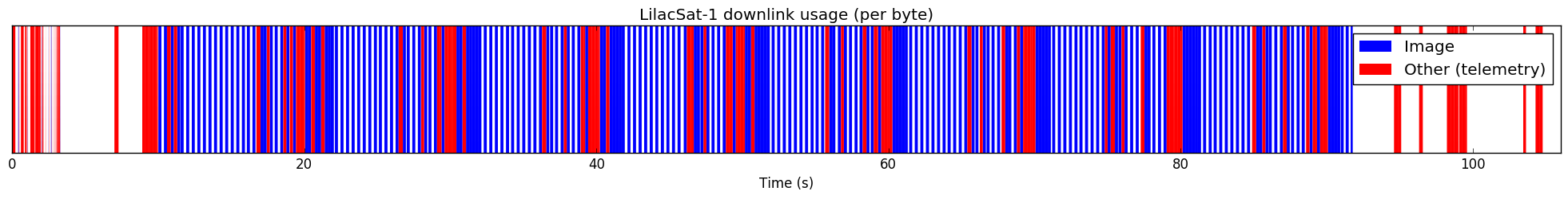
I have extracted the KISS stream from the recording and examined its usage to determine if it is being used at its full capacity or if it spends time idling. The image below represents the usage of each byte in the KISS stream, as time progresses. Bytes belonging to image packets are shown in blue, bytes belonging to other packets are shown in red and idle bytes are shown in white. (Remember that you can click the images to view them in full size).
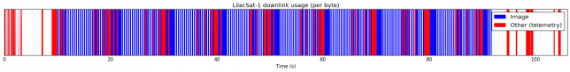
The first 3 or 4 seconds of the graph are garbage, since the signal wasn’t strong enough. Then we see some telemetry packets and the image transmission starts. We observe that most image packets are transmitted leaving an idle gap between them. The size of the gap is similar to the size of the image packet. Every 10 seconds, a bunch of telemetry packets are transmitted, in a somewhat different order each time. Some telemetry packets are sent back to back, and others are interleaved with image packets. Image packets are only sent back to back just after a telemetry transmission.
The next graph shows the usage of the KISS stream averaged over periods of 5 secons. The y-axis means fraction of capacity of the link, so a 1 means that the full 3400bps are used. The capacity spent for image packets is shown in blue and the capacity used for telemetry is shown in red. The green curve is the sum of the blue and red, so it means the fraction of time that the link is not idle. We see that the link is never used completely. The total usage ranges between 60% and 90%, but never reaches 100%.
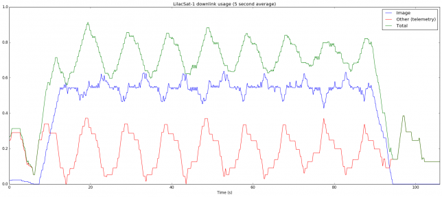
As expected, the capacity used for telemetry spikes up every 10 seconds. The blue curve is more interesting. It is roughly around 55%, but whenever telemetry is sent, it decreases a little. Just after each telemetry burst, the blue curve increases a little. This matches the behaviour we have seen in the previous graph. Every 10 seconds a telemetry burst is sent, using up some capacity that would normally be spent for image. After the telemetry burst, some image packets are sent back to back in a burst, peaking up to 60% capacity, but soon the packets continue being sent with idle gaps between them, and the capacity goes down to 55%.
It is a bit strange that the link is not fully utilised. One would expect that image packets are sent as fast as possible, stopping only to send telemetry. However, we have seen that there are many idle gaps. It seems that the image can’t be read very fast or that there is some other throttling mechanism. This would explain why a burst of image packets is sent after each telemetry burst: the image packets buffer up, because the link is sending telemetry. When the link is no longer busy with telemetry, it sends all the buffered image packets in a row, but soon enough image packets can’t be produced as fast as the link sends them, so idle gaps appear. This seems quite an important performance issue, as it appears that image transmission speed is capped at about 1870bps.
The Python code that generated these graphs can be seen below. The KISS file is also in the same gist.


