On March 22, CAMRAS performed a Venus radar experiment (or Earth-Venus-Earth bounce, as it is more commonly known in Amateur radio) in collaboration with Astropeiler Stockert, the Deep Space Exploration Society, and the Open Research Institute. The experiment was done in L-band, at 1299.5 MHz, using the 25 m Dwingeloo radiotelescope as transmitter and receiver and the Stockert 25 m telescope as a receiver. The experiment was done during the Venus conjunction, as this minimizes the distance between the Earth and Venus. The round-trip time to Venus was approximately 280 seconds. The radar waveform was a CW carrier with a duration of 278 seconds. It was transmitted a total of 4 times every 600 seconds. Thus each period was composed by:
- 278 second transmission
- ~2 second TX/RX guard time
- 278 second echo reception
- ~42 second wait
More transmissions were planned, including some spread-spectrum signals designed by the Open Research Institute. However, the transmitter started failing and they had to stop.
Update 2025-04-21: I have been informed that the spread-spectrum signal for this experiment was designed by CAMRAS. The waveform that the Open Research Institute is designing will potentially be used in future experiments.
CAMRAS has published an analysis of the recorded IQ data, showing successful echo detections with Dwingeloo and Stockert. There is an example Jupyter notebook that shows how to Doppler correct the echo and detect it with an FFT. All the recorded IQ data has been published.
In this post I will do my own analysis of the experiment. The goal is not to confirm the successful detection with an independent analysis, since I believe that the analysis published by CAMRAS is correct and leaves no doubt about this. It is to expand this analysis and to touch on other topics that this analysis has not covered:
- Calculation of the Doppler. CAMRAS has published CSV files containing the expected Doppler at each receiver, but they have not published the code to calculate this. Here I will do all the relevant calculations with SPICE.
- Doppler correction with the gr-satellites Doppler correction block, which performs linear interpolation of the Doppler frequency to calculate the frequency shift applied to each sample.
- High-quality spectral analysis with a polyphase filterbank.
- Try to estimate the Doppler spread and compare with some results in the literature.
Doppler calculations
Bistatic radar Doppler formula
Let us begin with how to calculate the Doppler for bistatic radar. We are interested in planetary radar, so we will need to take light-time delays into account. However, we will ignore relativistic effects. We denote the positions of the transmitter, target and receiver with respect to an inertial frame as \(x_T(t)\), \(x_0(t)\) and \(x_R(t)\) respectively. Since we are interested in calculating the Doppler correction that the receiver needs to apply, we begin at reception time \(t\) and work backwards. The light-time delay for the reflection path from the target to the receiver \(\tau_r(t)\) is the solution to the equation\[\tau_r(t) = \frac{1}{c}\|x_R(t) – x_0(t – \tau_r(t))\|.\]Likewise, the light-time delay for the direct path from the transmitter to the target \(\tau_d(t)\) is the solution to the equation\[\tau_d(t) = \frac{1}{c}\|x_0(t – \tau_r(t)) – x_T(t – \tau_r(t) – \tau_d(t))\|.\]The total time of flight is\[\tau(t) = \tau_d(t) + \tau_r(t).\]The Doppler frequency \(f_D(t)\) is \[f_D(t) = -\tau'(t) f_c,\]where \(f_c\) denotes the transmitted carrier frequency.
To compute \(\tau'(t)\), recall the formula for the derivative of the norm of a vector\[\frac{d}{dt} \|v(t)\| = \frac{\langle v'(t), v(t)\rangle}{\|v(t)|\|}.\]Using the notation\[e_r(t) = \frac{x_R(t) – x_0(t – \tau_r(t))}{\|x_R(t) – x_0(t – \tau_r(t))\|},\]and applying this to the equation for \(\tau_r(t)\), we obtain\[\tau_r'(t) = \frac{1}{c}\langle x_R'(t) – x’_0(t – \tau_r(t)), e_r(t)\rangle + \frac{1}{c}\langle x’_0(t – \tau_r(t)), e_r(t)\rangle \tau_r'(t).\]This gives the following formula to calculate \(\tau’_r(t)\):\[\tau’_r(t) = \frac{\langle x_R'(t) – x’_0(t – \tau_r(t)), e_r(t)\rangle}{c – \langle x’_0(t – \tau_r(t)), e_r(t)\rangle}.\]
In the same way, assuming that \(\tau’_r(t)\) has already been determined, we can compute \(\tau’_d(t)\). Using the notation\[e_d(t) = \frac{x_0(t – \tau_r(t)) – x_T(t – \tau(t))}{\|x_0(t – \tau_r(t)) – x_T(t – \tau(t))\|},\]and differentiating both sides of the equation that defines \(\tau_d(t)\), we get\[\begin{split}\tau’_d(t) = &\frac{1 – \tau’_r(t)}{c}\langle x’_0(t – \tau_r(t)) – x’_T(t – \tau(t)), e_d(t)\rangle\\ &+ \frac{1}{c}\langle x’_T(t – \tau(t)), e_d(t)\rangle \tau’_d(t).\end{split}\]Therefore, we get the following formula to calculate \(\tau’_d(t)\):\[\tau’_d(t) = (1 – \tau’_r(t))\frac{\langle x’_0(t – \tau_r(t)) – x’_T(t – \tau(t)), e_d(t)\rangle}{c – \langle x’_T(t – \tau(t)), e_d(t)\rangle}.\]Finally, \(\tau'(t)\) is computed as \(\tau'(t) = \tau’_d(t) + \tau’_r(t)\) using the two above formulas.
Computing bistatic radar Doppler with SPICE
Now let us see how to perform these calculations with SPICE. The key function that we will use is SPKEZR, which computes the state (position and velocity vectors) and light-time delay for a target with respect to an observer. This function is documented in more detail in the entry for SPKEZ, which is the same as SPKEZR but using integer codes instead of strings to specify the target and observer. Looking at the discussion of the reception case in the SPKEZR documentation we see that if we use "CN" as aberration correction, \(t\) as the observation time, \(x_0\) as the target, \(x_R\) as the receiver, and J2000 as the frame, the function will work as follows. First it will compute \(\tau_r(t)\) by iterating its definition formula until convergence, using \(\|x_R(t) – x_0(t)\|/c\) as the initial approximation. It will then compute the position vector\[y = x_0(t – \tau_r(t)) – x_R(t)\]and the light-time corrected velocity vector\[v = x’_0(t – \tau_r(t))(1-\tau’_r(t)) – x’_R(t)\](this is just the derivative of the position vector obtained by using the chain rule). It will return \(y\), \(v\) (as a 6-component vector), and the light-time delay \(\tau_r(t)\). Note that computing \(v\) involves first computing \(\tau’_r(t)\) (which is the value we actually want to calculate), but the documentation doesn’t explain how this value is computed, and it isn’t returned to the user.
We can now compute \(\tau’_r(t)\) by using the DVNORM function. This calculates the derivative of the norm of the position of a state \(y, v\) (where \(v = dy/dt\)) as\[\frac{d}{dt}\|y\| = \frac{\langle v, y\rangle}{\|y\|}.\]Applying the DVNORM function to the state \(y, v\) returned by SPKEZR and dividing by \(c\) we obtain \(\tau’_r(t)\), although not exactly in the way in which we had planned to calculate it above, since SPKEZR already calculated \(\tau’_r(t)\) internally.
To calculate \(\tau’_d(t)\), we use SPKEZR with an aberration correction of "CN", \(t – \tau_r(t)\) as the observation time, \(x_T\) as the target, \(x_0\) as the observer, and J2000 as the frame. This works as above, giving us the light-time delay \(\tau_d(t)\) computed by iteration, and the position vector\[z = x_T(t – \tau_r(t) – \tau_d(t)) – x_0(t – \tau_r(t)).\]The velocity vector considers the time \(s = t – \tau_r(t)\) as a fixed time that has \(ds/dt = 1\), rather than as a function of \(t\) having \(ds/dt = 1 – \tau’_r(t)\). Therefore SPKEZR returns the velocity\[w = \frac{dz}{ds} = x_T'(s – \tau_d(t))\left(1 – \frac{d\tau_d}{ds}(t)\right) – x’_0(s).\]Since we want \(dz/dt\), we need to multiply \(w\) by \(ds/dt = 1 – \tau’_r(t)\). This multiplication corresponds to the factor \(1 – \tau’_r(t)\) that we got in the above formula for how to compute \(\tau’_d(t)\). Thus, we can apply the function DVNORM to the vectors \(z\) and \((1 – \tau’_r(t))w\), and divide the result by \(c\) to obtain \(\tau’_d(t)\).
Note that we are always using "CN" as aberration correction rather than "CN+S". The correction "CN+S" also includes stellar aberration at the observer. This means that the apparent direction in which light rays arrive to the observer changes because of the velocity of the observer with respect to the solar system barycentre. For our purposes of Doppler calculations we are not interested in the apparent directions of arrival, so we omit the stellar aberration correction in most cases.
SPICE calculations for points on the surface of the target
The Doppler calculations can be done as described above with SPKEZR whenever the three objects involved (transmitter, receiver and target) are SPICE objects with an SPK kernel. For the transmitter and receiver, which are at fixed locations on Earth, we can create kernels using the pinpoint tool. We can use as target the SPICE object VENUS, which corresponds to the centre of Venus. This does not really correspond to the Doppler of any of the reflected signals, because they reflect off the surface of Venus, not the centre. However, as we will see, the Doppler for the centre of Venus is a good approximation for the Doppler at the sub-radar point.
To compute the Doppler for points on the surface of Venus, we could also use the pinpoint tool to define objects for them, by using coordinates with respect to the IAU_VENUS body-fixed frame. However, this is too limiting, because if we try to define many surface points, we will reach the limit of the SPICE object pool.
A better way to compute Doppler for points on the surface is to use the functions SPKCPT and SPKCPO. These behave similarly to SPKEZR, but allow defining either the target (SPKCPT) or the observer (SPKCPO) as a constant-position point with respect to a SPICE object. Therefore, instead of using VENUS with SPKEZR, we use SPKCPT and SPKCPO and specify the surface point by its coordinates in the IAU_VENUS frame.
Since Venus is modelled in SPICE as a sphere rather than an ellipsoid (Venus has a very slow rotation period, so its flattening is basically zero), the coordinates for points on the surface can be obtained by multiplying a unit vector by the radius of Venus. For a body with flattening we would need to use the function EDPNT instead, to compute the corresponding point on the surface of the ellipsoid.
Sub-radar point
Intuitively speaking, the sub-radar point is the intersection between the surface of Venus and the line joining the centre of Venus and the radar. The reflection at the sub-radar point is the one with less propagation time, so the sub-radar point echo is the first to arrive to the receiver. The radar wave arrives normal to the Venus surface at the sub-radar point (zero incidence angle), which gives the strongest reflection.
However, none of the above is exactly true once we take light-time delays into account. The concept of a sub-radar point is somewhat ill-defined. It might mean any number of things, which are not exactly the same:
- The point on the surface of Venus which is nearest to the receiver when observed at time \(t\). More formally, the point on the surface of Venus that emits photons at time \(t – \tau\) such that they arrive to the observer at time \(t\), and such that \(\tau\) is minimized subject to these conditions.
- The point on the surface of Venus that minimizes the total time of flight when observed at time \(t\). More formally, the point on the surface of Venus that reflects photons transmitted by the radar at time \(t – \tau\) such that they arrive to the observer at time \(t\), and such that \(\tau\) is minimized subject to these conditions.
- The point on the surface of Venus for which the scattering angle is zero when observed at time \(t\). More formally, subject to the condition that the reflection arrives to the receiver at time \(t\), the point on the Venus surface such that the scattering vector (the bisector of the apparent incoming and outgoing rays with respect to that surface point) is parallel to the surface normal at that point.
The distinction between these points barely matters in practice, since they are all quite close. Therefore, for practical reasons we use the first definition.
We use the SUBPNT SPICE function to calculate the sub-observer point on the Venus surface. This function is run with "INTERCEPT/ELLIPSOID" as method, VENUS as target, the time \(t\) as the observer time, IAU_VENUS as the body-fixed reference frame, "CN" as the aberration correction, and the radar receiver as the observer. This gives us the body-fixed coordinates of the surface point that is nearest to the receiver when observed at time \(t\). Once we have those coordinates, the remaining calculations are done as in the previous section.
Comparison with the CAMRAS CSV files
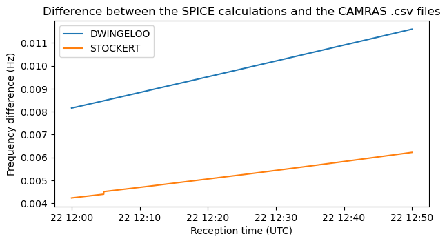
CAMRAS has published CSV files that list the expected Doppler at Dwingeloo and Stockert at reception times spaced by one second intervals. We can calculate the Doppler for the same reception times using SPICE and compare it with the CSV files. In this plot there is no appreciable difference.

If we compute and plot the difference, we see that it is just a few mHz. This is probably caused by me using slightly different coordinates for the telescopes. I got the coordinates by looking at the satellite view in Google maps, so they might be off by a couple metres. It is interesting that there is a jump in the Stockert difference. I don’t know what would cause this, other than a numerical error of some sort.
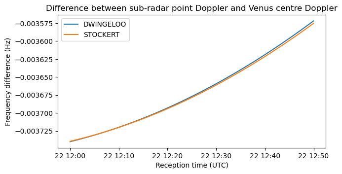
Additionally, we can plot the difference between the sub-radar point Doppler, calculated with SPICE as described above, and the Venus centre Doppler, also calculated with SPICE. The difference is also a few mHz, so we can ignore it for all purposes.
Doppler spread
Something I’m interested in is the Doppler spread that happens because different points on the surface cause different Doppler. To model this, besides the Doppler corresponding to each point on the surface, we also need to take into account the scattering angle. Points near the sub-radar point will have a strong reflection, while points close to the limb will have a much weaker reflection, since most of the energy hitting these points isn’t scattered back to Earth.
Given a reflection on the surface, the scattering vector is defined as the bisector of the incoming and outgoing rays. For best accuracy, these rays need to be calculated taking into account the stellar aberration correction for that point on the surface. This is the only place in this post where stellar aberration is used. The scattering angle is the angle between the scattering vector and the surface normal.
To compute the scattering angle for a given surface point with SPICE, we first use SPKCPT as before to compute \(\tau_r(t)\), since we need the reflection time \(t – \tau_r(t)\). Then we use SPKCPO at time \(t – \tau_r(t)\) with an aberration correction of "XCN+S", the radar receiver as target, and the surface point as observer to compute the apparent outgoing ray \(r_o\). We also use SPKCPO at time \(t – \tau_r(t)\) with an aberration correction of "CN+S", the radar transmitter as target, and the surface point as observer to compute the apparent incoming ray \(r_i\). To compute the scattering vector \(s\), we normalize \(u_o = r_o / \|r_o\|\), \(u_i = r_i / \|r_i\|\), and set \(s = (u_i + u_o)/(2 \|u_i + u_o\|)\). Since these vectors are in J2000 coordinates but we have the surface point in IAU_VENUS coordinates, we use PXFORM to calculate the rotation matrix from IAU_VENUS to J2000 at time \(t – \tau_r(t)\). Then we rotate the surface point coordinates to J2000 and normalize to obtain the surface normal \(n\). The scattering angle is the angle between the vectors \(s\) and \(n\).
I am using a HEALPix grid with a resolution of approximately 1 deg to calculate the scattering angle and Doppler at a grid of points on the surface of Venus. The following plot shows the scattering angle. The plot is centred on the sub-radar point, which has IAU_VENUS coordinates 9.5º S, 13.8º W. I am masking out points with a scattering angle greater than 90º, since those are points that the radar does not illuminate (they are on the back side of Venus as seen from Earth).
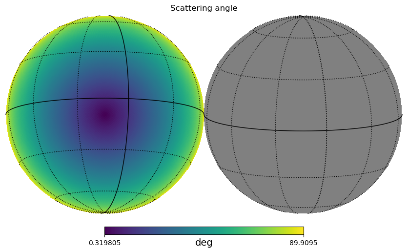
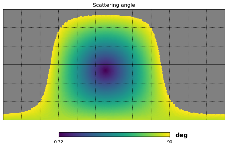
This provides a different view of the surface illuminated by the radar, by showing the surface of Venus in spherical coordinates.
The following plot shows the difference between the Doppler for each point on the surface and the Doppler for the centre of Venus.
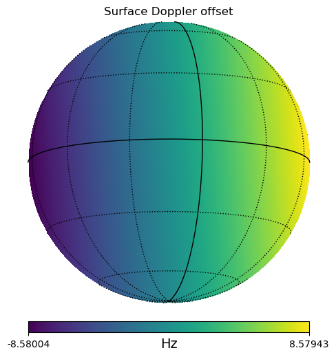
Unlike all other planets, Venus has retrograde rotation. This implies that the east limb approaches the observer, while the west limb recedes from the observer, explaining the signs in the figure above.
The following plot shows how the maximum and minimum surface Doppler change slightly over time.
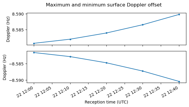
The equatorial rotational velocity of Venus is 1.81 m/s. Naïvely, we would expect a maximal surface Doppler offset of \(2 v_r f_c / c\), where \(v_r\) is the equatorial rotational velocity and \(f_c\) is the carrier frequency. This gives 15.7 Hz. So why is the maximum Doppler offset smaller? The reason is that Venus orbits around the Sun faster than the Earth. So there is a net velocity difference between Venus and Earth that is perpendicular to the line-of-sight vector (because the observation was done near the conjunction). You can picture Venus as if moving towards the right in the plot above. When pointing to surface points near the west limb, the line-of-sight is no longer completely perpendicular to this velocity vector. There is positive contribution to Doppler because of this, and this contribution cancels part of the negative Doppler due to the surface rotation. The opposite effect happens on the east limb.
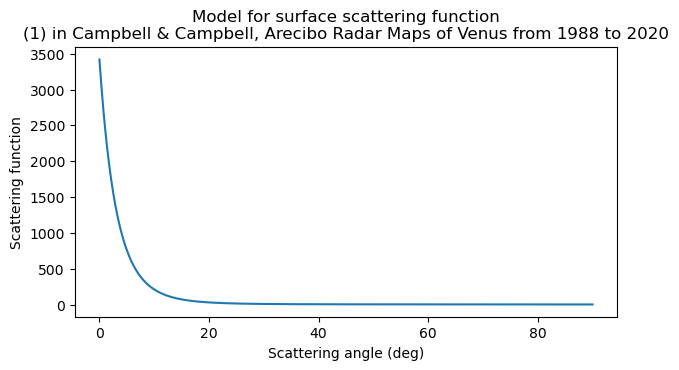
Besides the data above, we also need a model for how much power is reflected depending on the scattering angle. For this I have taken the model from equation (1) in the paper Arecibo Radar Maps of Venus from 1988 to 2020. This is an empirical model for OC (opposite circular polarization) scattering based on S-band observations at 2380 MHz. The model says that most of the power is reflected near the sub-radar point, with power quickly dropping for scattering angles above a few degrees.
We can use the model to compute an expected Doppler spread curve. This is done by taking a Dirac delta at the Doppler offset for each of the surface points I have calculated, scaling the Dirac delta by the scattering function corresponding to the scattering angle of that point, and convolving with a narrow Gaussian (\(\sigma\) of 0.1 Hz) to obtain a smooth function. The Doppler spread curve is normalized to a power of one at 0 Hz offset. We see that even though the maximum Doppler is 8.6 Hz, most of the power is concentrated within ±1 Hz.
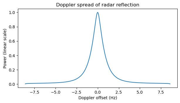
An important remark is that this Doppler spread has been obtained by using an empirical surface scattering model for 2380 MHz. At 1299.5 MHz the surface looks smoother. This means that scattered power concentrates more at lower scattering angles (a specular reflection off a smooth surface occurs only at a scattering angle of zero). Therefore, the real Doppler spread would be somewhat less than what predicted by this model.
Another paper that I have found about Venus Doppler spread is Radar Observations of Venus, 1961 and 1959. This corresponds to the earliest radar observations of Venus, done even before the rotation rate of the planet was determined (these observations contributed some data that supported the idea of a retrograde rotation). The observations were done at 440 MHz, a frequency at which the surface looks even smoother than at L-band. Figure 4 on the paper gives a Doppler spread concentrated on about ±0.4 Hz. To compare with our L-band spread, this needs to be scaled up by 1299.5/440, yielding ±1.18 Hz. However, this scaling doesn’t take into account the wavelength dependence of the scattering function.
High-quality PFB spectrum analysis
To analyze the IQ recordings done at Dwingeloo and Stockert I have decided to build a spectrum analyzer using a polyphase filterbank (PFB). The PFB will use channels with a width of 0.5 Hz and oversampling in frequency by a factor of 2. This means that the channel spacing is 0.25 Hz. The reason for oversampling by 2 in frequency is that this completely eliminates scalloping losses while still allowing channels to be summed to obtain a coarser frequency resolution. With no oversampling in frequency, typically the filter skirt will be at the edge of the channel. A CW carrier that falls exactly between two channels will appear in both channels, but reduced in power by the skirt. A way to solve this is to make the filter wider so that the passbands of adjacent channels overlap. However this causes a problem if we want to sum adjacent channels to decrease the frequency resolution by a factor of 2. The signals that appear in the overlapping area would be summed twice. With a factor of 2 oversampling in frequency we can solve all these limitations, as we will see.
The PFB will also do oversampling in time by a factor of 2. The reason for this is that with no oversampling in time, the signals that are on the skirt of the filter and past the edge of the channel will alias. They can potentially interfere with signals inside the channel, thus affecting the power measurement. With an oversampling in time by a factor 2, the skirt of the filter is not aliased, so the power measurement is accurate. If all these considerations about oversampling seem a bit confusing, they will perhaps make more sense when I discuss the details of the filter construction.
To build the PFB prototype filter I am using the pm-remez Python package, which is an implementation of the Parks-McClellan/Remez optimal FIR design algorithm that I wrote in Rust about a year ago. I am basically using the PFB example given in the pm-remez Python documentation. I start by designing a PFB filter for 1000 channels with 10 taps per channel. The IQ recordings are 5 ksps, so with a 0.25 channel spacing we will need 20000 channels. However, building a FIR of that size with the Remez algorithm is a very ill-conditioned problem, and pm-remez (and most other Remez implementations) will fail if requested to build such a filter directly. An approach that works well is to build a FIR with less channels, and then interpolate the impulse response to the desired number of channels, for instance using something as simple as linear interpolation. This approach is suggested in the pm-remez documentation.
The reason for using 10 taps per channel is that with less taps the filter shape doesn’t look too good. For a reasonable filter shape, at least 10 taps per channel are needed. We don’t want to make the filter too long either. The recording segments that we will process are 278 seconds long, and it is weird to process a data segment with an FIR filter whose impulse response has a length comparable to the data segment. At 0.25 Hz channel spacing and 10 taps per channel the impulse response is already 40 seconds long.
I have modified two things in the pm-remez PFB example. The first is that the example is for a PFB that is critically sampled in frequency (channel spacing is the same as channel width). Therefore, we need to multiply the cutoff frequency by 2 to obtain our oversampled PFB. The second thing is that I have added a way to adjust the cutoff frequency more finely. This is done to control the shape of the skirt of the filter, so that the skirts of every other bin overlap nicely and sum to a power close to one. We will see how this looks like below.
With a transition bandwidth of 12.5% (which is really 25% of the channel width due to how the way that oversampling in frequency has been fed into the filter design helper function), equal weights in the passband and stopband, and a \(1/f\) stopband response, pm-remez generates the following FIR. The passband ripple is great (less than 0.05 dB), and the \(1/f\) stopband response is a good idea for a PFB, because it reduces the integrated noise contribution from all the other channels. Furthermore, it allows us to design a filter that maybe doesn’t have a great rejection one channel away, but gets progressively better as we go further out in frequency.
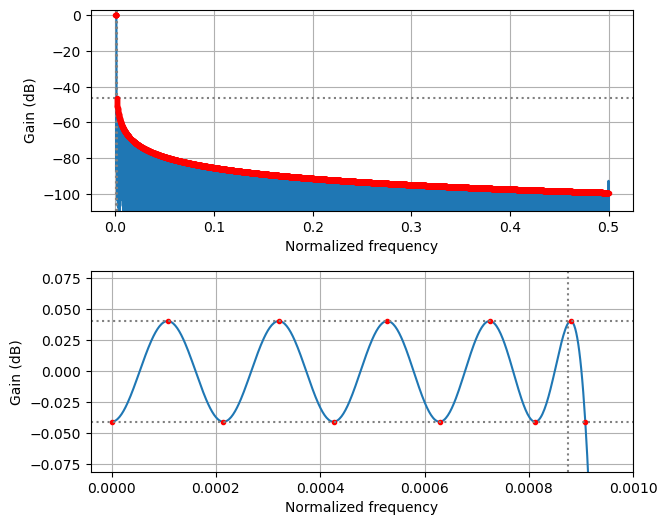
This is a detail of the frequency response on the first few channels. Note that since there is oversampling in frequency by 2, the cutoff is at the 1 channel mark, rather than the 0.5 channel mark. The stopband attenuation starts at -47 dB, which is not great, but due to the \(1/f\) response it becomes better than -60 dB after channel 5. For the analysis of these recordings, this PFB is quite reasonable, because we don’t have any strong signals in the spectrum that would leak to adjacent channels. Even a stopband rejection as poor as -30 dB would be fine.
To obtain the required prototype filter for 20000 channels, we simply interpolate linearly the impulse response of this FIR by a factor of 20. The response of the final PFB prototype filter looks pretty much the same as that of the 1000-channel filter when we look at a few channels near zero.
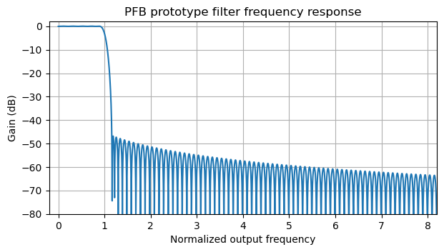
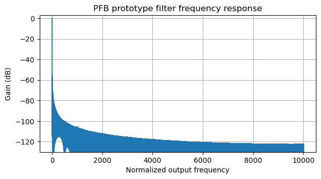
If we look at the full frequency response, we see that the \(1/f\) stopband response continues.
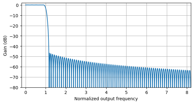
The following plot shows the frequency response of the first three channels of the filterbank. Note that channel 1 straddles channels 0 and channel 2, due to the oversampling in frequency. A signal that appears exactly at the edge of channel 0 will be somewhat attenuated in both channels 0 and 2, due to the transition band of their filters, but it will be fully present in channel 1.
We also plot the response of the non-coherent sums of the bins. These are \((|H_0(f)|^2 + |H_1(f)|^2 + |H_2(f)|^2)/2\) and \(|H_0(f)|^2 + |H_2(f)|^2\), where \(H_k(f)\) is the frequency response of channel \(k\). This non-coherent sum corresponds to the power that a signal at frequency \(f\) would cause if we compute the power it causes on each of the channels, and them sum the powers (either in the 3 channels and divide by 2, or only on channels 0 and 2).
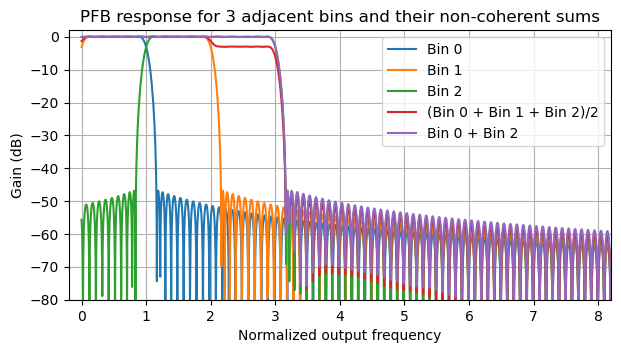
The location of the cutoff frequency of the filter has been adjusted by hand in such a way that the skirts of channel 0 and channel 2 are complementary and add up to something very close to one when doing this non-coherent combination. The consequence of this is that if we sum channels 0, 1 and 2 and divide by 2, we get a frequency bin with a response of 0 dB where two of these channels overlap (this is a 0.5 Hz region) and a response of -3 dB where only one of these channels is present (this is in two 0.25 Hz regions). Therefore, this gives a way of obtaining a coarser bin with a noise bandwidth of 0.75 Hz. Alternatively, we can sum channels 0 and 2. In this way we obtain a bin that is 1 Hz wide and is centred on channel 1.
In the following plot we can see a detail of the passband ripple of these non-coherent sums. We see that the skirts of the channels are well adjusted to achieve this complementary behaviour.
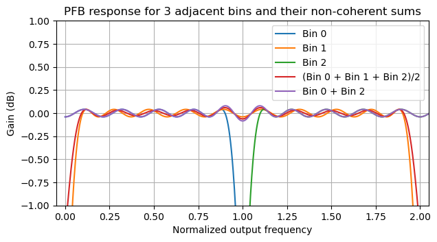
This property is useful because it allows us to average power in neighbouring bins as a way of reducing the noise variance, at the cost of decreasing the frequency resolution. When we do this, the effective filter shape we obtain is still nice, having a well-controlled passband. With other filter shapes we could either have dips in the response in channel edges (the typical case due to the skirt happening too soon), or peaks in the channel edges if the skirts overlap too much.
IQ recording processing
Initial inspection
The IQ recordings published by CAMRAS are 5 ksps. The original 1 Msps recordings are also available, but they provide no additional value to us because we are only interested in processing the CW signal, and the Doppler shift is just a few 100 Hz (I can imagine that the 1 Msps recordings were mainly intended for the spread-spectrum waveform).
The transmitted signal was RHCP, so the reflection is expected to be LHCP (most of the reflected power is in the opposite circular polarization). For Dwingeloo a single LHCP channel is given. For Stockert, horizontal and vertical polarization channels are given. CAMRAS says that these need to be combined with a phase shift of 260 degrees to obtain LHCP. We will self-calibrate on the reflected signal in order to check this.
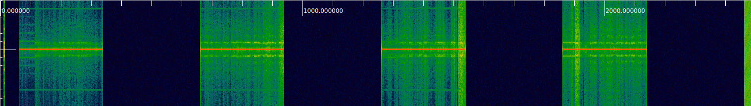
The Inspectrum waterfall for Dwingeloo can be seen below. The transmitted signal is visible because of leakage from the transmitter into the receiver. We can see a brief transmission at the beginning, which is the CW identification EVE25RD. Then there are the four 278 second tones and the reception intervals. At the right edge of the waterfall there is a wideband transmission. This looks like a transmission of the spread-spectrum waveform, which only lasted 56.3 seconds and was probably stopped because of transmitter problems. Later, and not visible in this part of the waterfall there is another CW transmission, lasting only 10.6 seconds. This was perhaps an automated transmission (since it started exactly at the 2640 second mark), or an attempt to test or troubleshoot the amplifier. Finally, there is a 2 second CW transmission almost at the end of the recording.
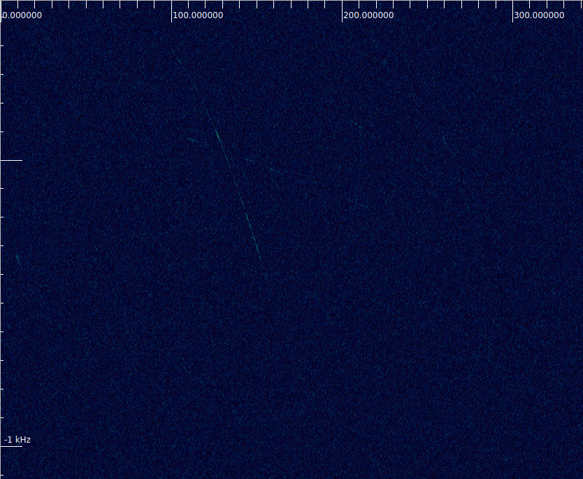
The waterfall of the Stockert recordings is interesting because we can see reflections with high Doppler drift when Dwingeloo is transmitting. The two stations are 250 km apart, so these are probably reflections off aircraft, or perhaps satellites (I highly suspect aircraft). These reflections are just a curiosity and they do not cause any problem for detecting the Venus bounce signal, since when that signal arrives back to Earth, Dwingeloo is no longer transmitting.
Doppler correction
Doppler correction of the recordings is done with the Doppler correction block from gr-satellites and a Doppler file that contains the expected Doppler at one second intervals. The Doppler file has been computed for the Venus centre using SPICE as described above. The Doppler correction block performs linear interpolation of the Doppler time series to compute the Doppler frequency at each sample. The error caused by this linear interpolation is bounded by\[\frac{\Delta^2}{8} \max \left|\frac{d^2 f_D}{dt^2}\right|,\]where \(\Delta\) is the time interval used in the Doppler time series. In this case,\[\left|\frac{d^2 f_D}{dt^2}\right| \leq 4.5\cdot 10^{-6}\ \mathrm{Hz}/\mathrm{s}^2,\]so using \(\Delta = 1 \mathrm{s}\) is perfectly fine, as it causes negligible interpolation error.
Extraction of the receive intervals
The four CW pulses are transmitted during the following intervals:
- 12:01:00 to 12:05:38
- 12:11:00 to 12:15:38
- 12:21:00 to 12:25:38
- 12:31:00 to 12:35:38
For each of these 8 timestamps, the corresponding time of reception at Dwingeloo and Stockert assuming a reflection at the Venus centre is computed using SPICE. This calculation uses "XCN" as the aberration correction on the Dwingeloo to Venus leg to compute the light-time delay of travel to Venus, and then "XCN" on the Venus to receiver leg to compute the light-time delay of travel back to the receiver.
To each of the expected reception times corresponding to these transmit timestamps we add/subtract a padding of \(2R_V/c\), where \(R_V\) denotes the radius of Venus, in order to enlarge the expected reflection interval to account for the different light-time delays to points in the surface. This is a minor and unimportant detail, since a padding of 40 ms applied to a 278 second interval hardly has any consequence.
The padded times of reception start and end are rounded to an integer sample index at 5 ksps, and these indices are used to extract 4 segments from each recording. Due to the rounding and the slightly different light-time delays, the length of some of the segments differs by one sample, so they are all zero padded to the same length.
Polyphase filterbank
The polyphase filterbank has \(N = 20000\) channels, so this is the FFT size that it uses. There are \(K = 10\) taps per channel. Since the polyphase filterbank is oversampled by a factor of two in frequency and also by a factor of two in time, each evaluation of the filterbank requires stepping the input by \(N/4\) samples. (The easiest way to realize this is that the output sample rate of each channel needs to be 1 sps, because the 0.5 Hz channels are oversampled by a factor of two in time. Therefore, one output sample needs to be produced in each channel for every \(5000 = N/4\) input samples).
Before applying the polyphase filterbank, each of the signal segments is zero padded both at the beginning and at end. At the beginning, \((K-1)N\) zeros are added. This has the consequence that the first filterbank evaluation has loaded in each arm \(K-1\) zeros and one sample of data. At the end, the segment length is first zero padded to an integer multiple of \(N\), and then \((2K-1-1/4)N\) additional zeros are appended. These zeros are added so that there are enough zeros after the signal to allow the polyphase filterbank to be evaluated with only one sample of the signal segment (zero padded to a multiple of \(N\)) on each arm, and \(K-1\) zeros from this additional padding, and then the filterbank can be stepped 3 times more (contributing an additional \(3N/4\) of padding). The next stepping of the filterbank would have no signal samples and be all zeros.
After doing this padding, the PFB can be evaluated in a relatively straightforward way by sliding an \(N\)-sample window in steps of \(N/4\) samples along the zero-padded input, and computing the convolutions of the window samples and the taps of each arm. These convolutions can then be all FFT’ed at the same time to obtain the filterbank output.
The filterbank output is an array of size \(3 \times 4 \times T \times N\), where 3 is the number of recordings that we are processing (one for Dwingeloo and two for Stockert), 4 corresponds to the four different transmissions, and \(T\) denotes the number of time samples produced by the PFB. The cross-correlation of the filterbank output is calculated by multiplying for each pair of recordings the filterbank output of one of them by the complex conjugate of the filterbank output of the other one. The cross-correlation is therefore an array of size \(3 \times 3 \times 4 \times T \times N\). We will mostly use the “diagonal” terms of this array (diagonal along the \(3 \times 3\) dimensions), which contain the power in each recording. But the off-diagonal term corresponding to the two Stockert recordings will allow us to combine coherently the two linear polarizations later.
Calibration
We perform an initial inspection of the PSD by summing up each of the diagonal cross-correlations along the time dimension (also accumulating together the 4 pulses). This already shows that the reflected CW carrier is visible in the spectrum of each recording. However, the recordings have different powers, so we need to calibrate this out.
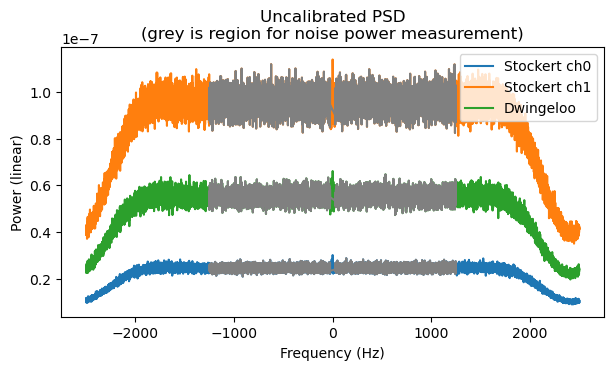
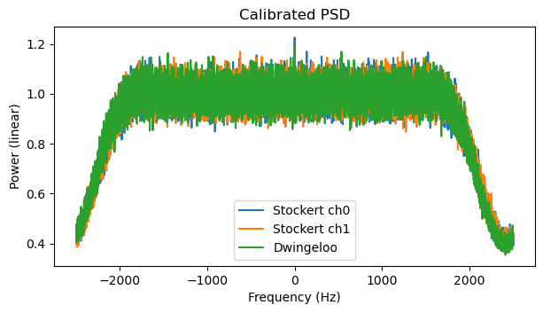
An area to measure the noise floor power is chosen by avoiding the centre of the spectrum (which contains extra power because of the CW carrier) and the edges of the passband. This area is shown in grey above. The average noise power in this area for each recording is computed. A gain factor for each recording is determined so as to make the average noise power equal to one. The gain factors are applied to the cross-correlation in order to calibrate it. The resulting calibrated PSDs now all have the same normalized noise floor level.
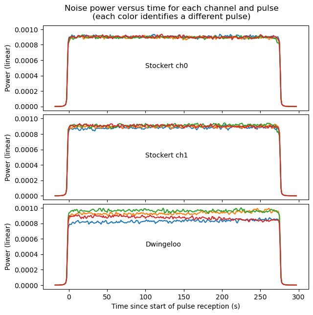
Another thing that we can look at is noise power versus time. For this, the same noise measurement area of the spectrum is used. Noise power is accumulated along the frequency dimension, and plotted here for each of the recordings and each of the pulses. We can see that Stockert ch0 has a very consistent gain over time. Stockert ch1 has a slightly less consistent behaviour, but it is still pretty good. Dwingeloo has large variations in power over time of up to 20%. I have decided to ignore this and not attempt to calibrate it out, since I cannot tell if the change in noise power is due to a change in gain, to a change in noise temperature, or a combination of both.
The next thing we do is to verify that the phase offset of 260 deg for the two Stockert channels given by CAMRAS is correct. For this, I accumulate the 4 pulses over time, sum the 5 central bins of the spectrum (-0.5 Hz, -0.25 Hz, 0 Hz, 0.25 Hz and 0.5 Hz), since those are the ones that contain most of the signal power, and look at the phase of the cross-correlation between Stockert’s ch0 and ch1. This gives an angle of 280 deg. This is relatively close to the 260 deg given by CAMRAS. Indeed, as shown by the figure below, there is little difference between using 280 deg or 260 deg to combine coherently ch0 and ch1. In what follows I will always use 280 deg to obtain a Stockert LHCP signal.
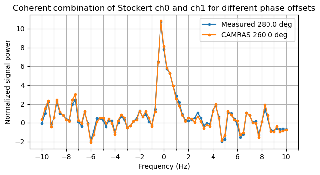
The plot above is a normalized spectrum. This is obtained by subtracting the average noise power over the noise measurement region of the spectrum and then dividing by the standard deviation of the noise in this measurement region. Therefore, in this normalized plot the noise is distributed as a normal with mean zero and standard deviation one. Detection values in \(\sigma\)’s can be read directly from the y-axis. So we see an \(11\sigma\) detection for Stockert in 0.5 Hz bandwidth.
Something else that I have looked at is whether there is any signal present in the cross-correlation between Dwingeloo and Stockert. I haven’t found any, and this is to be expected. The baseline between Dwingeloo and Stockert is \(10^6\) wavelengths. The corresponding angular resolution is 0.19 arcsec. The apparent size of Venus at conjunction is around 60 arcsec. Even though the area that produces most of the reflected power is smaller than the disc of the planet, it is still at least an order of magnitude larger than the angular resolution of this baseline. Therefore, this baseline resolves out the extended component of the reflection, and so the theory says that there should be little signal power in the cross-correlation. Besides, there is also the question of whether the coherence of the clocks of Dwingeloo and Stockert is good enough for us to be able to perform coherent integrations of tens or hundreds of seconds of duration in the cross-correlation.
Analysis
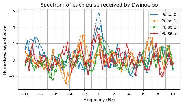
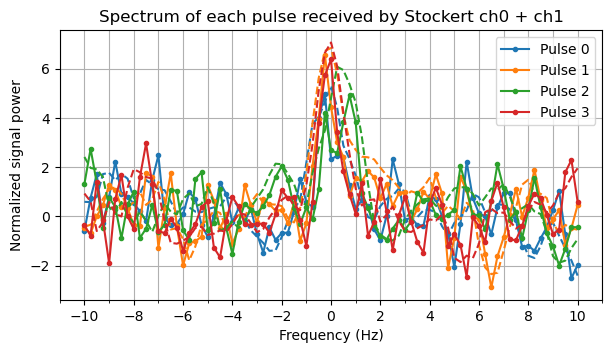
The following plots show the normalized spectrum of each of the four pulses as received by Dwingeloo and by Stockert (LHCP coherent combination). Besides the spectrum obtained with our 0.5 Hz binwidth, 0.25 Hz bin spacing PFB, a dashed line is shown that corresponds to a moving average of 5 frequency bins. Due to the remarks done above about summation of several PFB bins, we see that this moving average corresponds to sampling with a filter that has a 0 dB response in a 1 Hz region and a -3 dB response in two 0.25 Hz regions to the sides of this 1 Hz region. The total noise bandwidth of this filter is therefore 1.25 Hz.
We can already note something that CAMRAS also mentioned in their study. Dwingeloo has poorer receive performance. The signal is clearly detectable in pulses 0 and 3, but not in pulses 1 and 2. Interestingly, pulses 1 and 2 are the ones that have higher noise power, so this increase in noise power might be because of an increase in noise temperature rather than an increase in gain.
In Stockert each of the pulses can be detected individually.
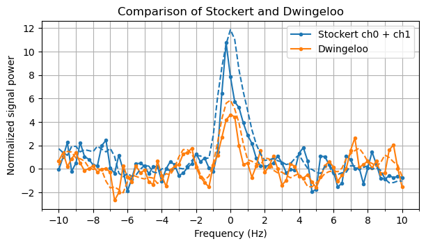
If we sum the four pulses together, we obtain the following spectra for Stockert and Dwingeloo. Stockert has a \(12\sigma\) detection in the smoothed spectrum (1.25 Hz noise bandwidth) and Dwingeloo only has a \(6\sigma\) detection in the smoothed spectrum.
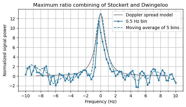
In order to measure the Doppler spread as best as possible, we perform a maximum ratio non-coherent combining of the spectra of Stockert and Dwingeloo. However, since the signal at Dwingeloo has 3 dB less than at Stockert, the maximum ratio combining doesn’t improve things by much. The plot below compares the maximum ratio combined spectrum with the model we had for the Doppler spread. We can see that the model predicts somewhat wider spread. Even after applying the 5-bin moving average, the measured spectrum is slightly narrower. Most of the signal power is contained in the 5 central bins. These occupy a 1.5 Hz area. So we can say that the measured Doppler spread is on the order of ±0.75 Hz.
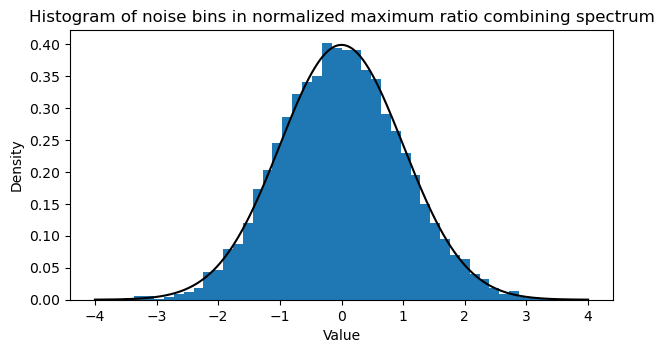
As a final check, the following shows the histogram of the bins in the noise measurement region of the normalized maximum ratio combining spectrum. Their distribution matches a normal quite well, so we see that there is no interference or other effects that disturb the noise statistics.
Code and data
All the materials used in this post can be found in this repository. This includes the Jupyter notebook used for all the analysis, as well as the GNU Radio flowgraph used for Doppler correction. The IQ files can be downloaded from CAMRAS here.
2 comments