This is a post I had announced since I first described Tianwen-1’s modulation. Since we have very high SNR recordings of the Tianwen-1 low rate rate telemetry signal made with the 20m dish in Bochum observatory, it is interesting to make detailed measurements of the modulation parameters. In fact, there is something curious about the way the modulation is implemented in the spacecraft’s transmitter. This analysis will show it clearly, but I will reserve the details for later in the post.
Here I will be using a recording that already appeared in a previous post. It was made on 2020-07-26 07:47:20 UTC in Bochum shortly after the switch to the high gain antenna, so the SNR is fantastic. The recording was done at 2.5Msps, and the spectrum can be seen below. The asymmetry (especially around +1MHz) might be due to the receive chain.
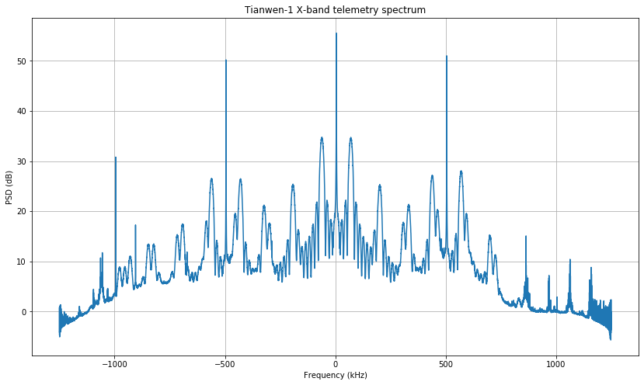
The signal is residual carrier phase modulation, with 16348 baud BPSK data on a 65536Hz square wave subcarrier. There is also a 500kHz ranging tone.
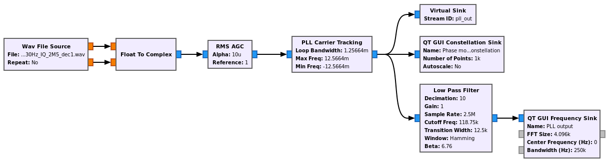
The detailed measurement of the modulation is done with this GNU Radio flowgraph. Since the flowgraph is quite large, I will explain it by sections. The first section is just used to lock a PLL to the residual carrier. There is an AGC with a very long time constant, in order not to damp out any possible amplitude modulation in the signal. Then a PLL with a bandwidth of 500Hz is locked to the residual carrier. Here the large bandwidth is not a problem, since the carrier is very strong.
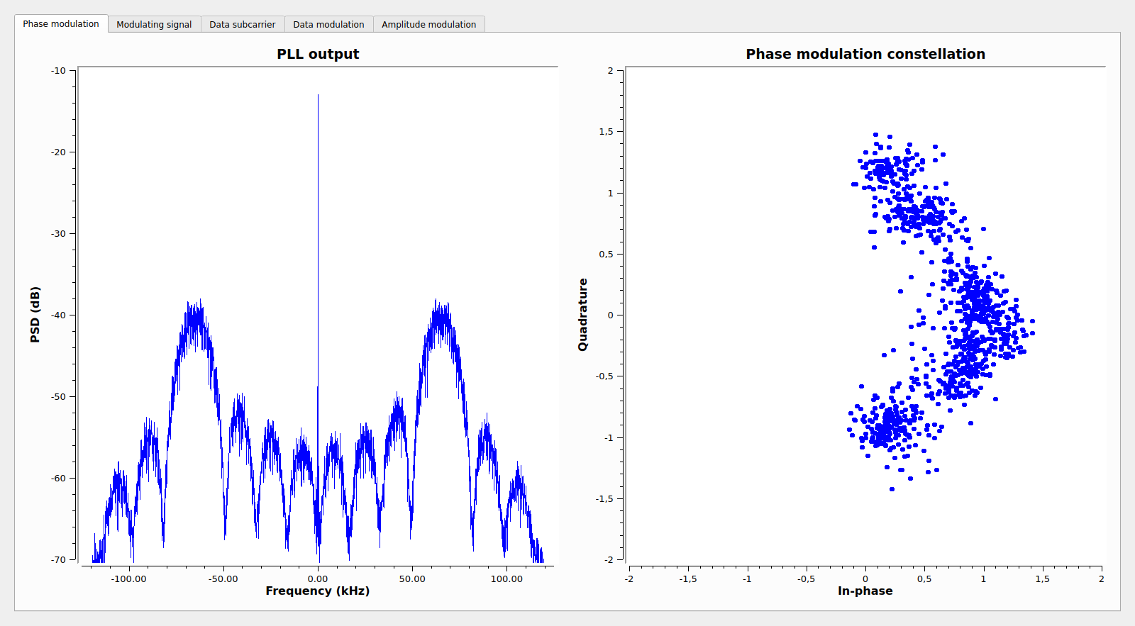
The GUI of the flowgraph is organized in tabs, since there are many GUI elements. The first tab is used to check correct carrier lock (note that only the central 250kHz of the modulation are shown in order to see the carrier better). We also show the constellation, which should look like an arc of circle symmetric about the point 1. However, we see that it is doesn’t have a perfect circular shape and it is somewhat asymmetric. This hints at some distortion in the form of amplitude modulation. As mentioned above, the distortion could be caused by the receiver.
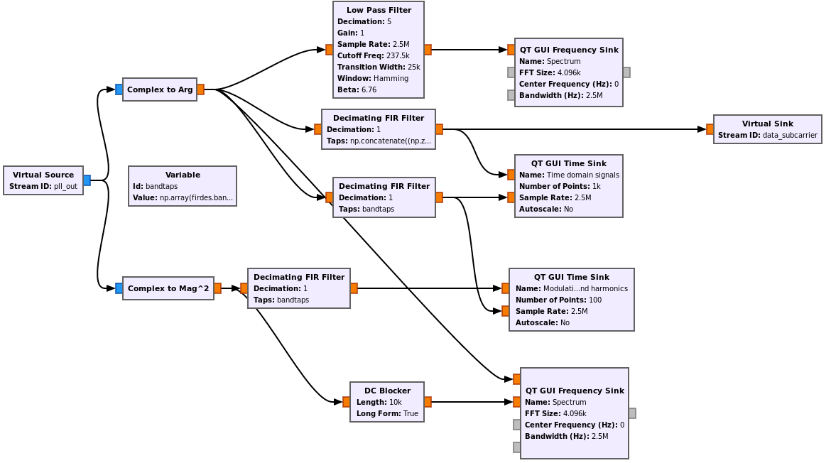
The next part of the flowgraph gets the phase and amplitude of the phase-locked signal. The spectrum of these two real signals is plotted. We expect to see the modulating signals in the phase and no amplitude modulation. The data subcarrier and ranging tone are separated by means of a narrow bandpass that only lets through the 500kHz tone and its 2nd harmonic at 1MHz.
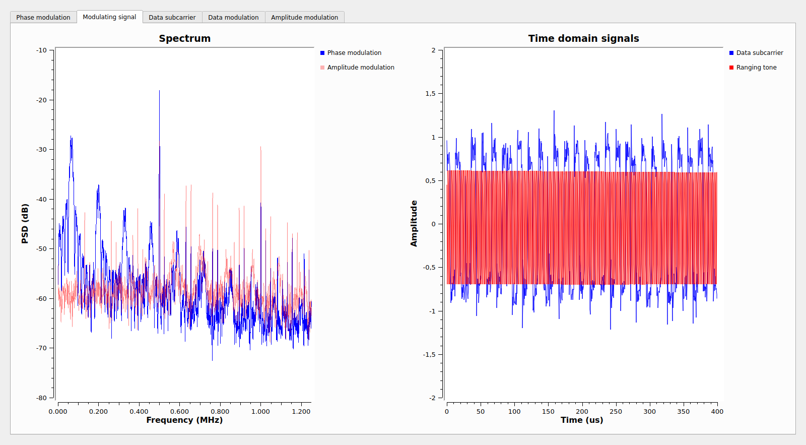
The output of this section can be seen below. In the spectrum of the phase modulation we see the BPSK data signal at 65536Hz and odd harmonics of the square wave subcarrier. We also see the 500kHz ranging tone and its 2nd harmonic some 22dB down. I don’t know why there is a 2nd harmonic, since there shouldn’t be regardless of whether the tone is a sine wave or a square wave. This might be caused by the signal distortion around +1MHz mentioned above. Most likely, in the undistorted signal the ranging tone is just a sine wave and there is no 2nd harmonic in the modulating signal (but the phase modulation will produce harmonics).
The amplitude modulation shows significant components at 500kHz and 1MHz, and a large number of spurs. The amplitude modulation will be investigated later.
The right hand side of the GUI shows the separated data and ranging signals in the time domain. The deviation of the data modulation (which will be measured later) is 0.725 radians. This is slightly less than \(\pi/4\), but it includes some possible losses in the measurement, so the real deviation might be \(\pi/4\). The deviation of the ranging tone is around 0.75, so again near \(\pi/4\). When both the data modulation and the ranging tone coincide, the total deviation is near \(\pi/2\), which agrees with the constellation shown above.
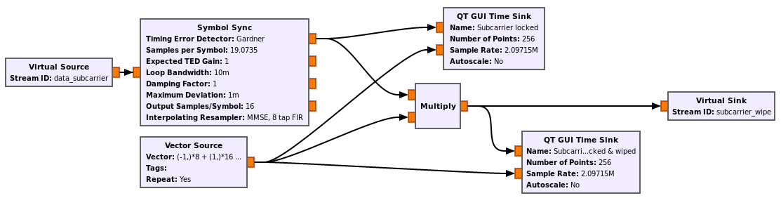
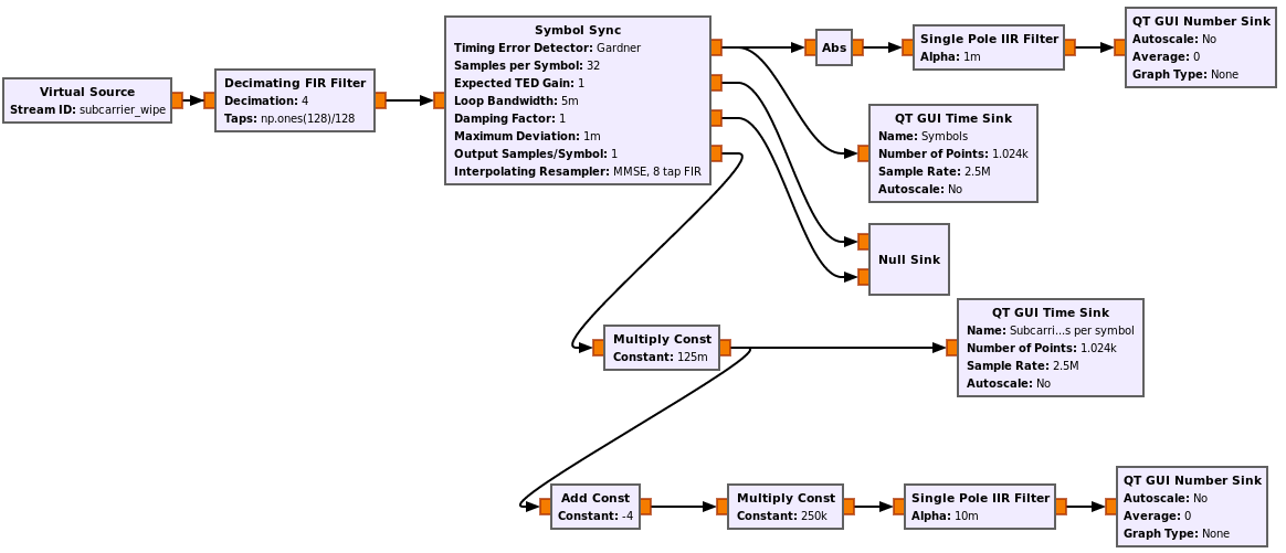
The next part of the flowgraph is used to investigate the relation between the BPSK symbol clock and the square wave subcarrier. To do so, we use the Symbol Sync block to lock to the subcarrier and output at 16 samples per symbol, so we get 32 samples per subcarrier cycle. An artificial subcarrier square wave is then generated at 32 samples per cycle and multiplied by the signal in order to wipe the subcarrier off and leave only the BPSK data modulation.
The figures below show the curiosity about the signal I mentioned at the start of this post. In this GUI tab we plot the following. In the upper left we show the data and subcarrier signal. There is no symbol shaping, so both the data and subcarrier are square waves. The subcarrier frequency is four times the baudrate, so there are four subcarrier cycles per symbol. This is what in the GNSS literature is called BOC(4) (GNSS isn’t directly related to deep-space communications but shares many similarities with these modulations). There are 8 subcarrier cycles plotted, so we have a total of two symbols. The red trace is a reference that shows what should the subcarrier look like in the absence of a data modulation.
The upper right plot is like the left one except that the waveform is multiplied by the reference subcarrier in order to remove the subcarrier and leave only the BPSK data modulation. Finally, the bottom plot shows the spectrum of the signal, from DC up to the 3rd subcarrier harmonic.
Now we note something interesting. If you look at the upper right plot, you’ll see that the BPSK symbol changes precisely at an edge of the reference subcarrier. This can also be seen in the Data + Subcarrier waveform in the upper left plot. There is a very short spike, but other than this the change in the BPSK symbol looks like a change in the phase of the subcarrier. We change from a subcarrier that has the same sign as the reference subcarrier to a subcarrier which has the opposite sign.
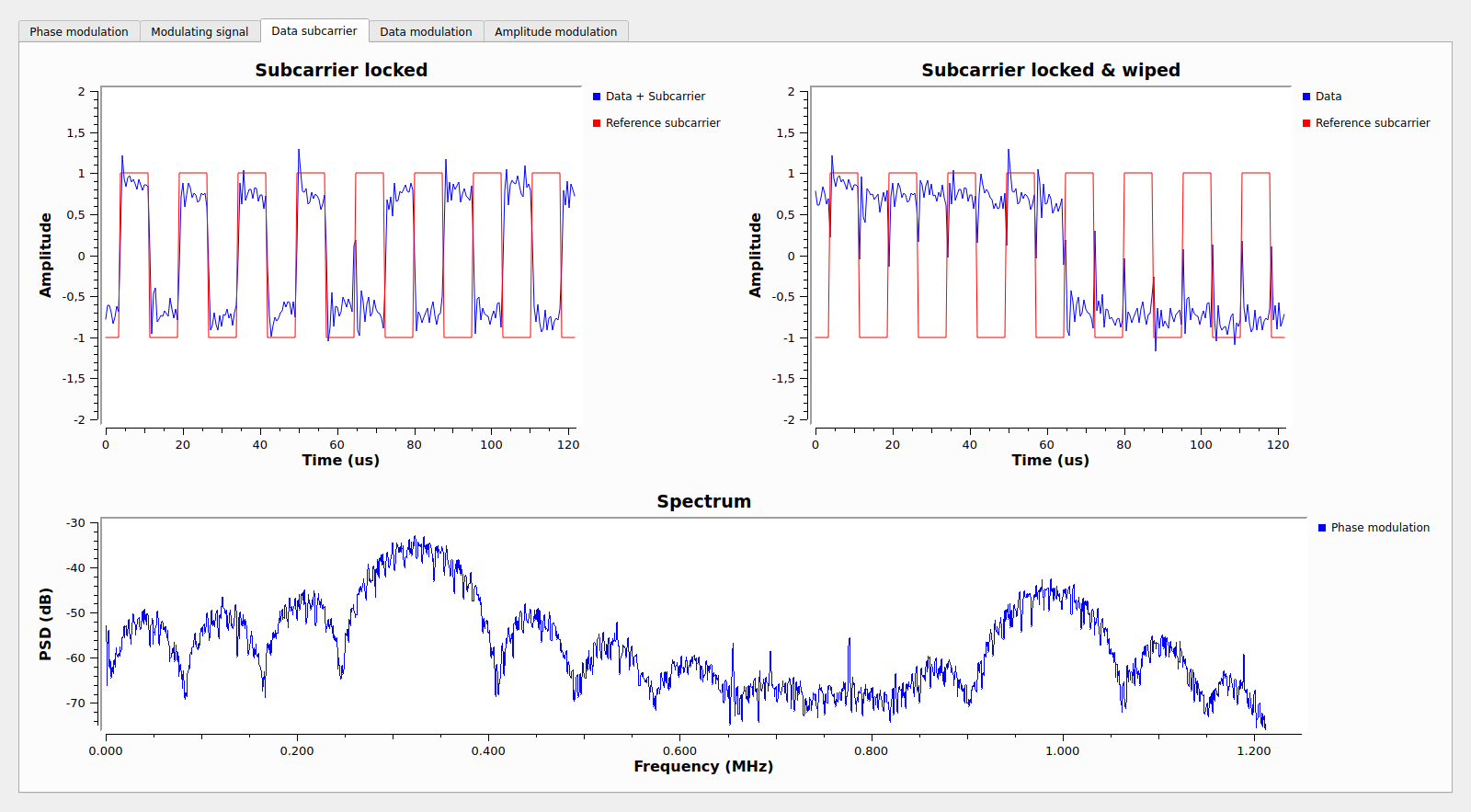
All the properties shown above happen because the subcarrier clock and the symbol clock are in-phase: the symbol changes happen at an edge of the subcarrier. This is called BOC-sine or BOCsin in the GNSS literature. However, this situation doesn’t maintain for long. Interestingly, it happens that in Tianwen-1 the subcarrier clock and symbol clock are generated from independent oscillators. These means that the frequency ratio is not exact and the clocks slide against each other.
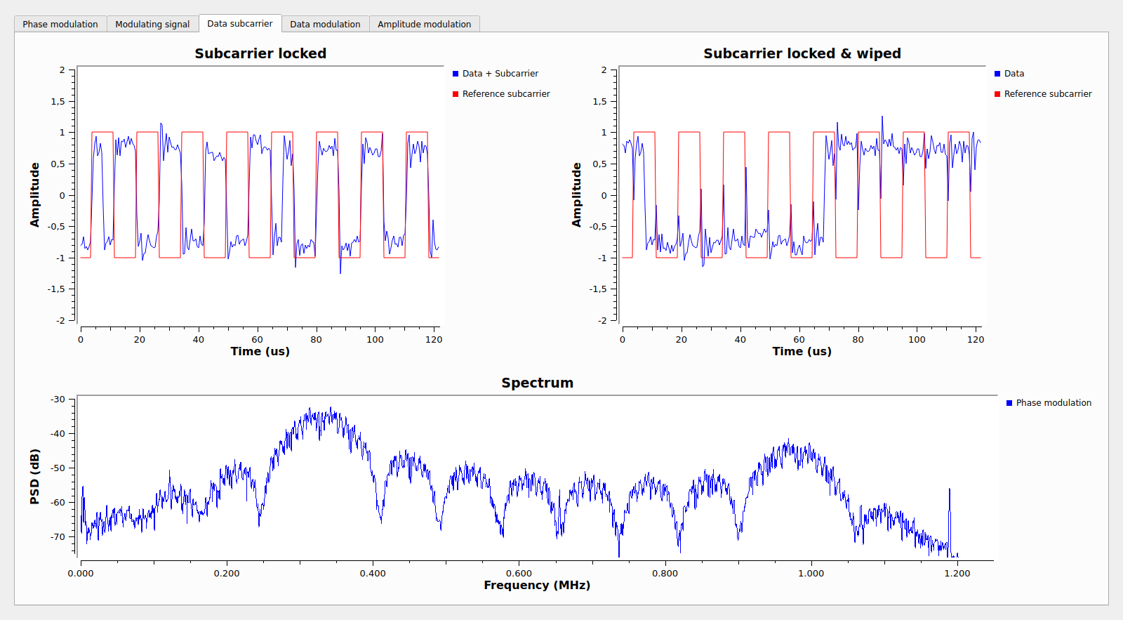
In this particular recording, the period of the symbol clock is slightly larger than 4 subcarrier cycles. The effect in these plots is that the symbol transition keeps crawling to the right until eventually it happens in the middle of the subcarrier edges. This is shown below.
The subcarrier and symbol clocks are now in quadrature, and this modulation is called BOC-cosine or BOCcos in the GNSS literature. In the upper left plot we can see that the symbol change in the middle of the subcarrier edges produces one cycle of a square wave of frequency twice the subcarrier.
It is also interesting to compare the spectrums for the in-phase and the quadrature situations. When the subcarrier and symbol clock are in phase, the low frequency sidelobes between DC and the main lobe at 65536Hz have more power. When the subcarrier and symbol clock are in quadrature, the higher frequency sidelobes between the main lobe and the 3rd harmonic have more power.
As the subcarrier and symbol clocks keep sliding, the modulation keeps changing smoothly between the in-phase and quadrature configurations, exchanging power between the low frequency and higher frequency sidelobes. In this particular recording this happens every 1.4 seconds approximately, but we have seen other periods, since the clocks are free-running.
The video below shows the flowgraph GUI running so that you can watch how the symbol edges crawl slowly towards the right and how the power of the sidelobes alternates between the lower and higher frequency sidelobes. For this video, a throttle block was used to play the signal 10 times slower than real time.
The constant change between the in-phase and quadrature configurations produces a characteristic pattern in the signal when seen in a waterfall plot. Achim Vollhardt DH2VA called this “dancing”. See his tweet, which includes a short video. This effect also appears in the waterfall images posted by other Amateurs, such as Ferruccio IW1DTU.
The next and final section of the flowgraph performs clock recovery on the BPSK data signal (with the subcarrier already wiped off). Since the symbol pulse shaping is square, a square filter is used as a matched filter.
This is mainly used for two applications. First, to do a precise measurement of the amplitude of the symbols, which corresponds to the deviation of the data subcarrier, minus any small implementation losses. Second, for a measurement of the frequency difference between the symbol clock and the subcarrier clock. This section of the flowgraph works locked to the subcarrier clock, so any rate deviation of the recovered symbol clock from its nominal value indicates a frequency difference between the two clocks.
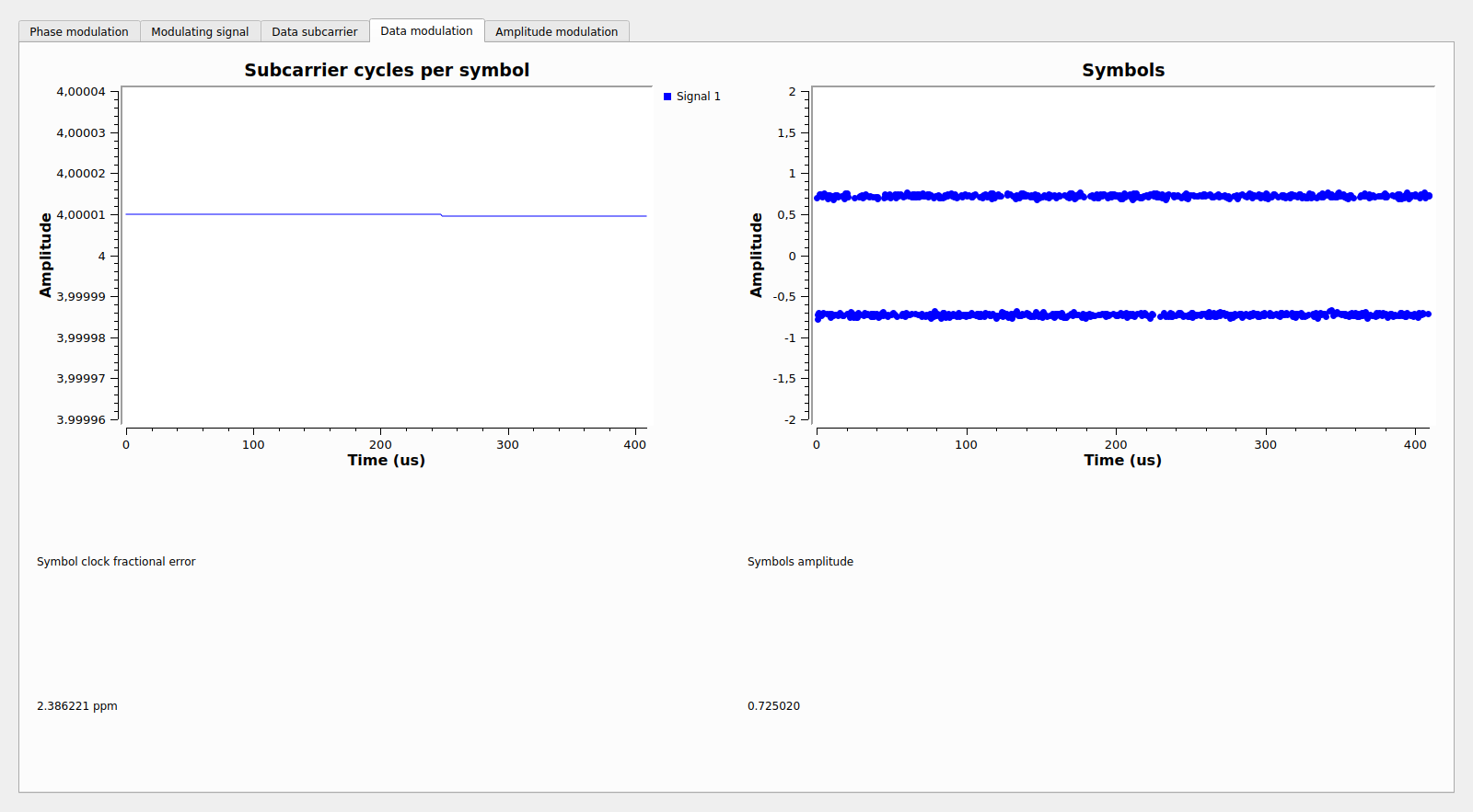
The GUI of this section of the flowgraph is shown here. We see that the symbols have very little noise due to the high SNR of the recording. The average amplitude of the symbols is around 0.725, as remarked above.
The precise measurement of the symbol clock fractional error is difficult, since this parameter probably varies with time. The value is around 3ppm. By doing the math, we see that with this frequency error, the configuration will change between in-phase and quadrature every 1.27 seconds.
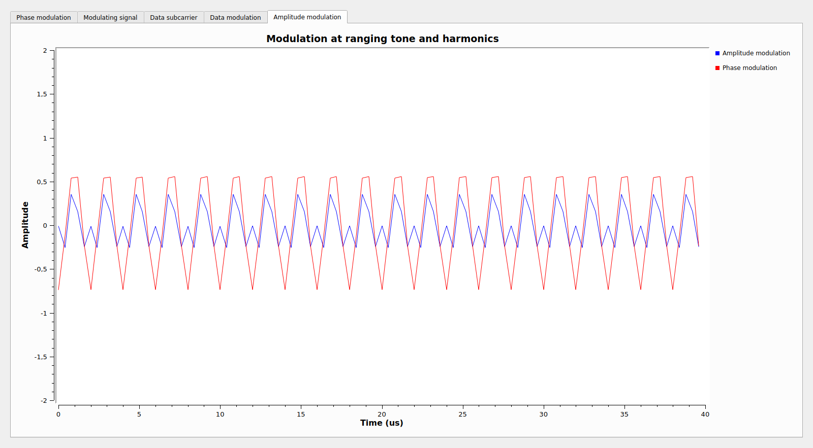
Finally, there is a GUI tab that tries to show the amplitude modulation and relate it to the phase modulation of the 500kHz ranging tone. Both are passed through a narrow bandpass filter than only lets 500kHz and 1MHz through, since otherwise it is difficult to see any patterns in the time domain of the amplitude modulation. Since the signal distortion that causes amplitude modulation is probably at the receiving end, it is not easy to draw any definitive conclusions from this plot.
Hi. What subcarrier wave means here? As you know, we first modulate our data with BPSK modulation using Pulse shaping, and then PM Modulation is done, now what is the subcarrier rule?
Hi David. I don’t understand your question. The modulation described here is PCM/PSK/PM this means that data is BPSK modulated onto a subcarrier.
You right, when we use from sine or square subcarrier, it means that after PCM/PSK/PM , the carrier of the signal shift using sine or square subcarrier.
Or not, before PM modulation this subcarrier is applied on BPSK signal. Which one is true?
The data is BPSK modulated at 16384 baud on a (real) 65336Hz square wave. The resulting real signal is then used to phase modulate an RF carrier at X-band.