Last week I did an experiment where I transmitted WSPR on a fixed frequency for several days and studied the distribution of the frequency reports I got in the WSPR Database. This can be used to study the frequency accuracy of the reporters’ receivers.
I was surprised to find that the distribution of reports was skewed. It was more likely for the reference of a reporter to be low in frequency than to be high in frequency. The experiment was done in the 40m band. Now I have repeated the same experiment in the 20m band, obtaining similar results.
In a previous post I discussed my BER simulations with the LilacSat-1 receiver in gr-satellites. I found out that the “Feed Forward AGC” block was not performing well and causing a considerable loss in performance. David Rowe remarked that an AGC should not be necessary in a PSK modem, since PSK is not sensitive to amplitude. While this is true, several of the GNU Radio blocks that I’m using in my BPSK receiver are indeed sensitive to amplitude, so an AGC must be used with them. Here I look at these blocks and I explain the new AGC that I’m now using in gr-satellites.
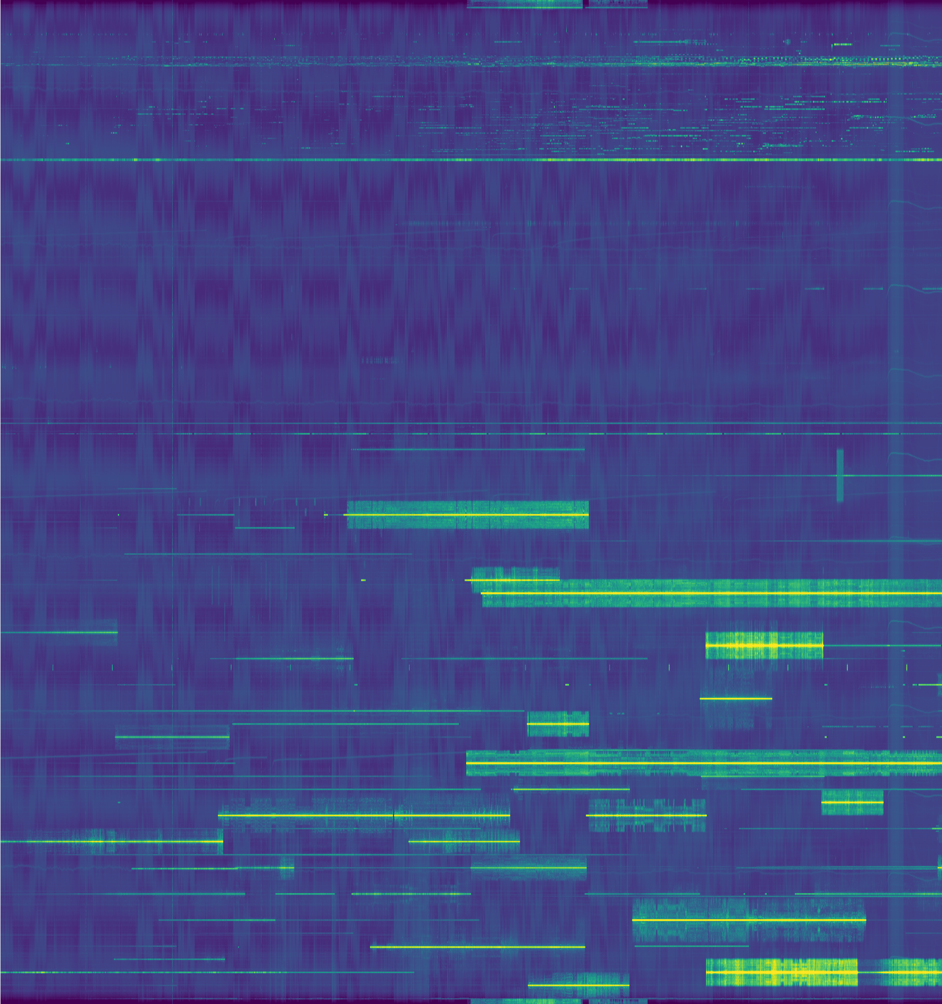
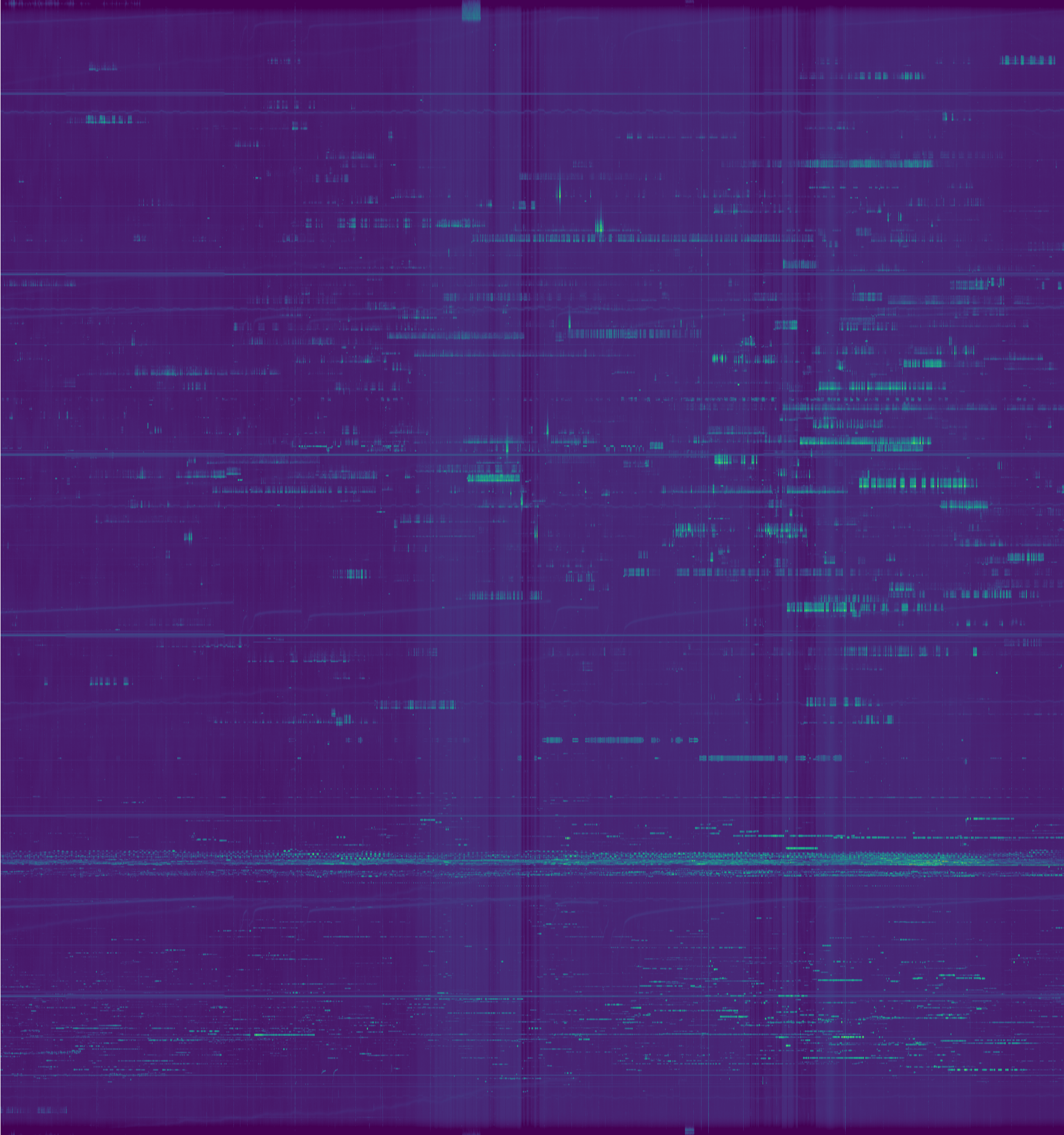
Meanwhile, I have used a variation of my usual Python script to plot waterfalls of the recording. Below you can see waterfalls for the 3 bands. They use the same scaling, with a dynamic range of 50dB, so it is easy to see how the noise floor changes per band. The carriers of the strongest broadcast AM stations are clipped. The resolution in these waterfalls is 187.5Hz or 15s per pixel.
40m waterfall (centre frequency 7180kHz)30m waterfall (centre frequency 9970kHz)20m waterfall (centre frequency 14175kHz)
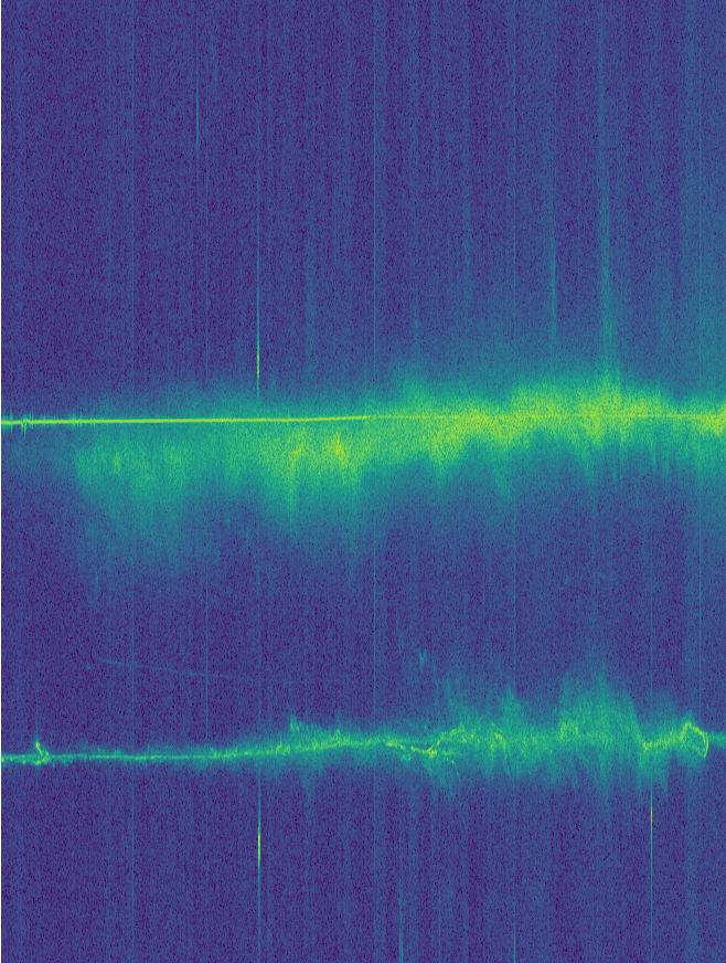
I have also taken a high resolution waterfall around the WWV carrier at 10MHz. The resolution is 22.9mHz or 65.5s per pixel, and the frequency span is 19.95Hz.
Centre frequency: 10MHz. Span 19.95Hz.
Near the centre of this waterfall, two signal can be seen. The signal which is concentrated in frequency is leakage from my 10MHz GPSDO. The signal which is spread out in frequency is the carrier of WWV, probably mixed with BPM. I’m not sure about the identity of the signal below them, which is about 5Hz below 10MHz. I suspect that it is JN53DV.
This waterfall shows that the 500ppb TCXO of my Hermes-Lite 2.0beta2 is stable to a few tens of parts per billion, as I remarked in my WSPR study.
More than a year ago, I spoke about my efforts to decode ÑuSat-1 and -2. I got as far as reverse-engineering the syncword and packet length, and I conjectured that the last 4 bytes of the packet were a CRC, but without the scrambler algorithm I couldn’t do much. Recently I’ve been exchanging some emails with Gerardo Richarte from Satellogic, which is the company behind the ÑuSat satellites. He has been able to provide me the details of the protocol that I wasn’t able to reverse engineer. The result of this exchange is that a complete decoder for ÑuSat-1 and -2 is now included in gr-satellites, together with an example recording. The beacon format is still unknown, but there is some ASCII data in the beacon. Here I summarise the technical details of the protocol used by ÑuSat. Thanks to Gerardo for his help and to Mike DK3WN for insisting into getting this job eventually done.
Over the last few days I’ve been transmitting WSPR on 40m with 20dBm of power using my Hermes-Lite 2.0beta2. For this, I’m using the instrument output of the Hermes-Lite, which is driven by an OPA2677 200MHz dual opamp that produces a maximum output of 20dBm. I’ve been transmitting always on the frequency 7040100Hz. I have been collecting the reports from the WSPR database for a total of 2518 reports over 5 days of activity.
There are many statistics that can be done with this data, but since I have always been transmitting on the same frequency, it is quite interesting to look at the frequency in the reports. My Hermes-Lite is quite stable in frequency, as it uses a 0.5ppm 38.4MHz TCXO from Abracon. In fact, in the shack its stability is usually much better than 0.5ppm. During these tests I have verified the accuracy of the Hermes-Lite frequency by receiving my DF9NP 27MHz PLL, which is driven with a DF9NP 10MHz GPSDO. The 27MHz signal is usually reported around 3Hz high by the Hermes-Lite, with a drift of roughly 0.3Hz. This accounts for an error of 0.1ppm, and the drift is around 10ppb.
It seems that this performance is much better than the usual performance of the Amateur radio transceivers that report on the WSPR network, so the frequency reports can be used to measure the error of the frequency references in these Amateur radio transceivers. Noting that at 27MHz my Hermes-Lite is 3Hz low in frequency, I have determined a correction of -0.782Hz for my WSPR frequency, so I have chosen to take my transmission frequency as 7040099.218Hz when doing the calculations. This is probably accurate to a few tens of ppb.
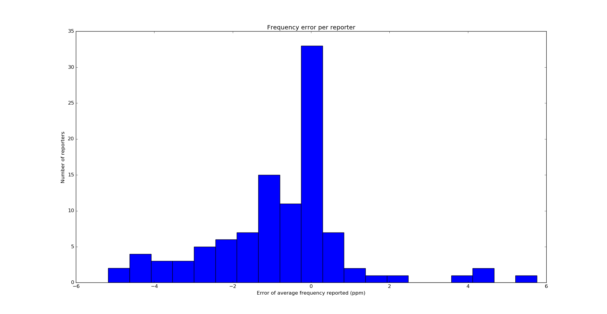
I wanted to do a statistic of the distribution of the error in the frequency references of the WSPR receivers. To do this, I’ve decided that it’s better to first do, for each reporter, an average of the frequency of its reports, and then take this average as the frequency measured by that reporter. Then I do a histogram of the errors in the frequency reported by each reporter. The first average is done because there are some reporters which have a great number of reports with a very similar frequency (because their receiver might have an error, but it doesn’t drift much), and so the histogram would be biased with these reports if I just plotted the histogram of all the frequency reports. The histogram is shown below.
Frequency error of WSPR reporters
I find this histogram rather surprising. I expected to get a normal distribution or something similar, or at least a symmetric histogram centred on an error of 0ppm. However, the histogram is clearly skewed to the left. We conclude from this that a good number of WSPR receivers are quite accurate in frequency, and have an error of 0.5ppm or less. However, from those that are not accurate, it is much more probable that they are low in frequency (so they report me at a higher frequency).
I still have to find a good explanation for this effect. However, I have suspicions that this has something to do with the way that the frequency of a quartz crystal depends on the temperature (and this depends on the way that the crystal is cut). I have found in this document the image below.
Note that non-AT-cut crystals are low in frequency over most of the temperature range, so I can’t help but think that this is too much of a coincidence with the skew in my histogram above. Other people have pointed out that this is not so simple, as for instance the adjustment of the tuning capacitors of the crystal oscillator also plays an important role. It would be good to repeat this test in other bands and by other stations, perhaps in other parts of the world (my reporters come from Europe) and see if they also obtain a skewed histogram.
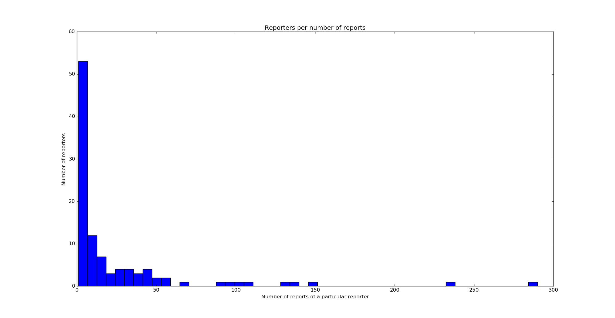
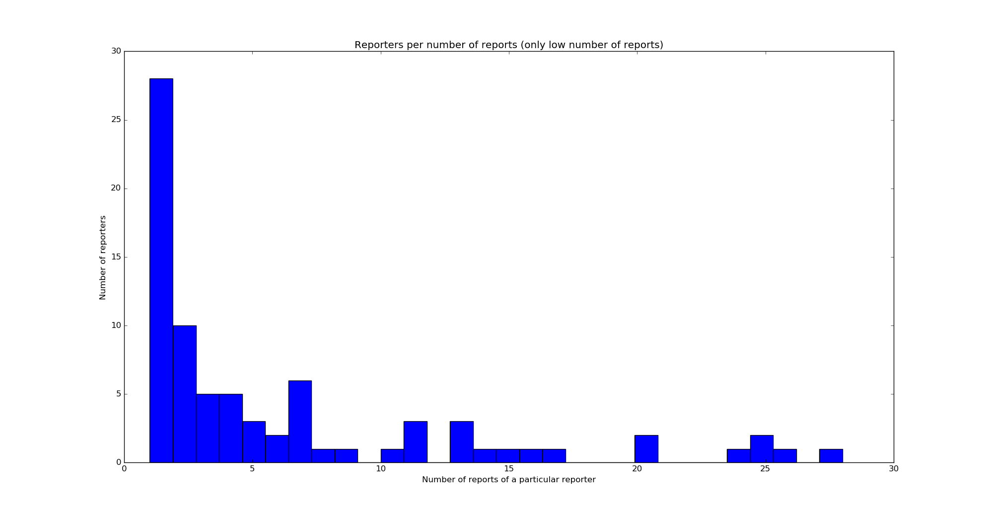
As an indication of the statistical significance of this test, I can say that a total of 2518 reports coming from 104 different reporters have been used. Just looking at these numbers is very far from doing a proper hypothesis contrast, but it is indicative that I have used a good amount of data. It is also interesting to look at the distribution of the number of reports given by each reporter. This is shown in the two histograms below (first for all numbers of reports and then for 30 reports and less).
The Python script and data used in this post are in this gist.
Lately, I have been playing around with the concept of doing acquisition and wipeoff of JT9A signals, using a locally generated replica when the transmitted message is known. These are concepts and terminologies that come from GNSS signal processing, but they can applied to many other cases.
In GNSS, most of the systems transmit a known spreading sequence using BPSK. When the signal arrives to the receiver, the frequency offset (given by Doppler and clock error) and delay are unknown. The receiver runs a search correlating against a locally generated replica signal which uses the same spreading sequence. The correlation will peak for the correct values of frequency offset and delay. The receiver then mixes the incoming signal with the replica to remove the DSSS modulation, so that only the data bits that carry the navigation message remain. This process can be understood as a matched filter that removes a lot of noise bandwidth. The procedure is called code wipeoff.
The same ideas can be applied to almost any kind of signal. A JT9A signal is a 9-FSK signal, so when trying to do an FFT to visually detect the signal in a spectrum display, the energy of the signal spreads over several bins and we lose SNR. We can generate a replica JT9A signal carrying the same message and at the same temporal delay than the signal we want to detect. Then we mix the signal with the complex conjugate of the replica. The result is a CW tone at the difference of frequencies of both signals, which we call wiped signal. This is much easier to detect in an FFT, because all the energy is concentrated in a single bin. Here I look at the procedure in detail and show an application with real world signals. Recordings and a Python script are included.
In a previous post, I spoke about the cubesat D-SAT. The thing that first caught my attention about this satellite is its image downlink and the quality of some of the images that Mike DK3WN has managed to receive. Yesterday, Mike sent me an IQ recording of D-SAT downlinking a couple of images. After using the Groundstation software by the D-SAT team to verify that the images in the recording can be decoded, I have reverse engineered the protocol used to transmit images and added an image decoder to the D-SAT decoder in gr-satellites.
The image decoder can be tested with the dsat-image.wav recording in satellite-recordings. This WAV file contains the image below, which shows the Southwestern part of Spain and Portugal. The image was taken by D-SAT on 2017-08-17 10:09:54 UTC and received by Mike during the 19:10 UTC pass that evening.
Image of Spain and Portugal taken by D-SAT
According to the TLEs, at the time this image was taken, D-SAT was just above Rincón de la Victoria, in Málaga, passing on a North to South orbit. This means that D-SAT’s camera was pointing more or less in a direction normal to the orbit.
This image is a 352×288 pixels JPEG image with a size of 13057 bytes. It took 43 seconds to transfer using D-SAT’s 4k8 AF GMSK downlink (yes, the overhead is around 100%, more on that later). In the rest of this post, I detail the protocol used to transmit the images.
Back in September 26 2016, I posted an email in Spanish to the Hamnet.es mailing list detailing my proposal for an IPv6 Amateur radio network, and trying to engage people into some preliminary tests. In October 1 2016, I posted a summary (in English) of my message to the 44net mailing list. There was some discussion afterwards in the list, but no real actions were taken. Since then, no much interest in IPv6 for Amateur radio seems to have sprung. Still, I think that the time for IPv6 will come. I have collected my IPv6 for Amateur radio proposal in a page here for future reference. At least I hope that this pops up on Google searches for IPv6 and Amateur radio, since there is not much material about this on the Internet, and most of what one can find is quite dated.
D-SAT is an Italian cubesat that will demonstrate a new deorbit hardware. Apparently this system uses dedicated propulsion to make the satellite re-enter from a 500km orbit in 30 minutes. It also carries three more experiments and it was launched in June 23 together with several other small satellites. According to the information from the team, it transmits 4k8 telemetry in the 70cm band. It is not stated explicitly, but we read attentively, we see that it uses a NanoCom U482C transceiver from GOMspace.
Recently, I have seen Mike DK3WN decode very nice images from D-SAT and I have investigated a bit to see what software he is using.
The satellite team provides some decoding software through their forum, which requires registration. Version 2 of their software can be downloaded directly here using the password dsatmission. Its software is based on GNU Radio and it uses a few components from gr-satellites, namely the U482C decoder and some KISS and CSP blocks. These have been incorporated into their decoder from before gr-satellites was restructured. They include a note thanking me in the README, but I didn’t ever hear from them that they were using gr-satellites. It would have been nice if they had contacted me, since this opens up many possibilities for collaboration.
Apart from that, they include a groundstation software which performs telemetry decoding and so on. Unfortunately, the groundstation software is closed-source, distributed only as an x86_64 Linux executable. This is not good for Amateur Radio. We should strive for open source software and open specifications for everything that transmits in our bands. The groundstation software is also distributed in a quite ugly manner as the remains of an Eclipse project (source code stripped, of course). However, it is interesting because it seems that this software is the same they use in their groundstation, and it supports sending commands to the satellite. Naturally, the command transmission is not implemented in the software they distribute, but it is still very interesting to have a peek and see what kinds of commands the satellite supports.
I have added a D-SAT decoder to gr-satellites. The decoder supports sending frames to their groundstation software. Here I describe how to set everything up.
Several weeks ago, in an AMSAT EA informal meeting, Eduardo EA3GHS wondered about the possibility of using WSJT-X modes through linear transponder satellites in low Earth orbit. Of course, computer Doppler correction is a must, but even under the best circumstances we cannot assume a perfect Doppler correction. First, there are errors in the Doppler computation because the TLEs used are always measured at an earlier time and do not reflect exactly the current state of the satellite. This was the aspect that Eduardo was studying. Second, there are also errors because the computer clock is not perfect. Even a 10ms error in the computer clock can produce a noticeable error in the Doppler computation. Also, usually there is a delay between the time that the RF signal reaches the antenna and the time that the Doppler correction is computed for and applied to the signal, especially if using SDR hardware, which can have large buffers for the signal. This delay can be measured and compensated in the Doppler calculation, but this is usually not done.
Here we look at errors of the second kind. We denote by \(D(t)\) the function describing the Doppler frequency, where \(t\) is the time when the signal arrives at the antenna. We assume that the correction is not done using \(D(t)\), but rather \(D(t – \delta)\), where \(\delta\) is a small constant. Thus, a residual Doppler \(D(t)-D(t-\delta)\) is still present in the received signal. We will study this residual Doppler and how tolerant to it are several WSJT-X modes, depending on the value of \(\delta\).
The dependence of Doppler on the age of the TLEs will be studied in a later post, but it is worthy to note that the largest error made by using old TLEs is in the along-track position of the satellite, and that this effect is well modelled by offsetting the Doppler curve in time. This justifies the study of the residual Doppler \(D(t)-D(t-\delta)\).