Interested by the forthcoming HamSci December 2021 eclipse festival of frequency measurement, I have decided to enable and test the external 10 MHz input of my Hermes-Lite 2 DDC/DUC HF transceiver. This will allow me to use a GPSDO (the Vectron MD-011 which has appeared in other posts) to reference the Hermes-Lite 2 in order to measure frequency accurately.
My Hermes-Lite 2 is a beta2 unit that I built by hand. Most of the options aren’t installed, since I decided that I would install these options if and when I wanted to use them. Therefore, to use the external clock option I have first needed to install a few components.
The Hermes-Lite 2 uses the VersaClock 5P49V5923 as clock synthesizer to generate the 76.8 MHz sampling clock. Usually, a 38.4 MHz TCXO (X2 in the schematic) is used. It is connected to the XIN_REF pin of the VersaClock, and the VersaClock is used as a frequency doubler.

When using an external 10 MHz clock, the input clock is supplied to the VersaClock using the CLKIN pin and the VersaClock performs a multiplication by 192/25 to generate the 76.8 MHz sampling clock.
To use the external clock input I have installed CL1 (the SMA connector), B58 (an AC coupling cap), and R39 and R40, which are used as a voltage divider so that a 3.3V LVCMOS clock is reduced to approximately 1Vpp. This divider comes straight from the datasheet.
The instructions to enable the 10 MHz external clock from software are here. There is some cleverness involved in both the fact that it’s necessary not to ever stop the VersaClock output, since it’s used as clock in most of the FPGA, including the I2C control of the VersaClock, and also the best way to configure the VersaClock registers to achieve the required multiplication ratio. I haven’t looked at these in any detail, since everything has worked as expected.
These days, the Python code to enable the external clock is included in this hermeslite.py module and can be easily called whenever it’s needed from a Juyter notebook, even if other applications are using the Hermes-Lite 2.
The MD-011 GPSDO that I’m using produces a 10 MHz sine wave output. I wasn’t sure if this was going to work with the VersaClock, since the data sheet says that a square wave is required and lists a minimum and maximum slew rate for the square wave. Using a sine wave isn’t mentioned at all in the datasheet. However, it seems that this works fine. The sine wave ends up as a 1Vpp sine at the VersaClock CLKIN pin, and the VersaClock has no problem locking to it.
The first thing I have verified is whether the VersaClock is doing an exact multiplication by 192/25 or just some other ratio which is very close but not quite exact. A typical issue with fractional-N synthesizers is that the multiplication factors they generate involve very large numerators and denominators that approximate the factor you want, but are not exact. This causes a frequency error. Knowledge of the exact value of this frequency error is needed to correct it at some point in the measurement chain.
In this case, it turns out that the VersaClock is doing the exact multiplication by 192/25. The figure below shows the test I did for the multiplication factor. The yellow channel is hooked up to the VersaClock 76.8 MHz output, while the blue channel is hooked up to the MD-011 1PPS output. The trigger is done on the rising edge of the 1PPS. If the 76.8 MHz output is an integer number of Hz, then we will see that the yellow trace is stationary. Otherwise the yellow trace will drift by at whatever rate corresponds to its fractional Hz part. Note that persistence is turned up so that we can see any drift that would happen.

This doesn’t completely prove that the multiplication factor is exactly 192/25, since the output may well be 76800001 Hz, or anything else that is an integer number of Hz close to 76.8 MHz. However, when we have fractional-N synthesis errors, the frequency error we get is very rarely an integer number of Hz (and often the error is less than 1 Hz). Therefore, this test gives good evidence that we have the exact multiplication factor we want. It also shows that the VersaClock is correctly locked to the 10 MHz input and that its output doesn’t have high jitter or other problems.
Another thing that can be seen with this test is that the phase relationship between the 76.8 MHz output and the 1PPS edges changes when the Hermes-Lite 2 is power cycled. This is to be expected. In theory there are 25 different phase relationships in which a 76.8 MHz clock can be coherently locked to a 10 MHz clock, because the multiplication factor is 192/25 when written as an irreducible fraction. Therefore, even though the 10 MHz output of the GSPDO has a fixed phase relationship to the 1PPS output, the 76.8 MHz won’t have a fixed deterministic phase relationship to the 10 MHz clock. This is not important for frequency measurement, but if we were interested in very precise timing measurements involving the sampling clock, we would need to be aware that the sampling clock edges might be off from the 1PPS by a non-deterministic error of up to ±6.5 ns (half a sample period).
The next test is to validate frequency measurement with GNU Radio. There are two things that need to be handled here to get accurate measurements. First, the local oscillator frequency of the DDC receiver will not be exactly what we want. This happens because the local oscillator is driven with an NCO, which has a quantization in the frequencies it can generate. We need to know the frequency error of this NCO so that we can correct for it.
The second thing is lost packets. Regardless of how we measure frequency, in the end we will measure phase difference versus time, and time is measured by counting IQ samples from the SDR. If we lose packets, the time count will be wrong and this will cause an error in the measurement of any frequencies that are not at DC in the SDR IQ output. Therefore, it is important to account for lost packets, since even if infrequently, there are going to be some lost packets. It is easier to handle these correctly than to try to engineer the system so that no packets are lost.
Regarding the DDC local oscillator frequency, the simplified version of how this works is that a 32-bit NCO is used in the FPGA, so the frequency quantization is \(76.8/2^{32}\) MHz. To compute the frequency error we let \(x = 2^{32}f/(76.8\cdot 10^6)\), where \(f\) is the frequency in Hz we want to set the NCO to. Then we put \(y = \text{round}(x) – x\). The NCO error is \(2^{-32}y\cdot76.8\cdot10^6\) Hz.
More in detail, the software sends the NCO frequency in Hz as a 32-bit integer (see this documentation), so that only integer Hz frequencies can be commanded. The FPGA computes the rounded control word for the NCO in the following way. The 32-bit frequency \(f\) is multiplied by \(M_2 = 2^{57}/(76.8\cdot10^6)\), rounded to an integer, and \(M_3 = 2^{24}\) is added (see here and here). Then the 25 LSBs of the result \(M_2 f + M_3\) are discarded and the next 32 bits are taken as the control word of the NCO (see here). The goal of adding \(M_3\) is to perform rounding half-up. However, looking at these more closely we see that the rounding error in \(M_2\) might affect the result by changing slightly the points at which rounding changes from down to up. Therefore, in some cases the result we get might deviate from the simplified description given above, and in these cases we should use \(y + 1\) or \(y – 1\) instead of \(y\).
As an example, for \(f = 30000007\) Hz, the FPGA computes the NCO control word 1677721992. However, the exact calculation of the NCO control word would give \(x =\) 1677721991.468. This should be rounded down to 1677721991 rather than up as the FPGA does. However, the amount of frequencies \(f\) for which the FPGA does not round as expected is small (only 8% for \(f\) on the order of 10 MHz, and 23% for \(f\) on the order of 30 MHz; it is proportional to \(f\)). Also, nice round frequencies will typically have the expected rounding. Thus, we’re unlikely to encounter this unexpected roundings in practice, but we can do the same calculation as the FPGA to be sure of what the FPGA is doing (since otherwise we would get a frequency error in our measurements).
To handle lost packets, I have modified gr-hermeslite2 so that when it detects that some ethernet packets have been lost (using the sequence counter in the Metis protocol packets), it inserts fake packets filled with zeros to account for the lost IQ samples. By doing so, from the perspective of GNU Radio there are no lost samples and everything works as expected, besides the fact that we have a few samples with zeros where a gap due to lost packets would happen. The modifications are already in the master branch of the repository. It has been a bit tricky to get this working correctly because the original code that handled the sequence counter had a bug: it didn’t detect any lost frames after the sequence counter rolled over, since it didn’t account for the fact that the sequence counter only uses 20 bits rather than 32.
The screenshot below shows the GNU Radio flowgraph I’m using for frequency measurement. In this experiment, in order to validate that everything is working as it should, we measure the 10 MHz output of the GPSDO. Since the Hermes-Lite 2 is locked to this 10 MHz clock, we should measure exactly 10 MHz. The 10 MHz from the GPSDO is leaked into the Hermes-Lite 2 RF input by using a short antenna connected to the Hermes-Lite 2. This already gives us a fairly strong signal that we can measure.
The GNU Radio flowgraph can be downloaded here. It uses GNU Radio 3.8, since I haven’t ported gr-hermeslite2 to GNU Radio 3.9 yet.
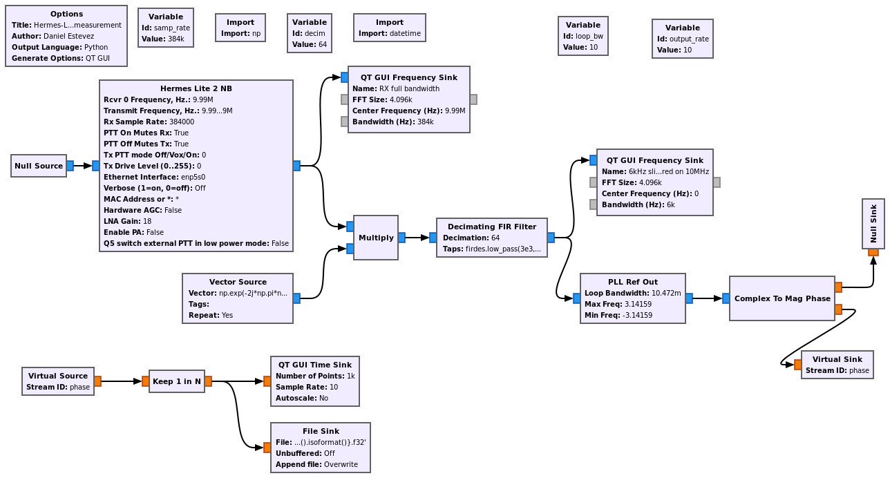
In order to test that the handling of lost packets is correct, the Hermes-Lite 2 is tuned to 9990 kHz, so that the 10 MHz signal appears at 10 kHz in the IQ output of the Hermes-Lite. By doing this, if there is any problem with lost or extra IQ samples, we will see the phase of the 10 kHz signal jump, whereas if we tuned the Hermes-Lite 2 to 10 MHz, then the signal would be at DC in the IQ output and we wouldn’t see any phase jump.
First we downconvert the signal at 10 kHz to baseband. In order to do so without having any numerical precision errors in the phase of the 10 kHz local oscillator that would accumulate over time, we generate our local oscillator as a periodic signal using the Vector Source. We are using a sampling rate of 384 kHz at the IQ output of the Hermes-Lite 2, so our Vector Source consists of a repeating vector of 384 samples that amounts to 10 cycles of a 10 kHz complex exponential.
After multiplication by this local oscillator, filtering and downsampling to 6 ksps, we use a PLL to measure the phase of the signal. The PLL Ref Out block locks to the signal under measurement and provides a “clean” output reference of which we can measure the phase. A bandwidth of 10 Hz is used in this PLL.
Finally, the phase measurements are downsampled so as to obtain a measurement rate of 10 Hz. The results are saved to a file and also plotted in the time domain.
Note that since the local oscillator of the Hermes-Lite 2 DDC is not exactly 9990 kHz, but rather has an error of some mHz, the signal we are measuring with the PLL doesn’t have a frequency of exactly 0 Hz, but rather of a few mHz. Therefore, we will see the phase measurements slowly changing with time.
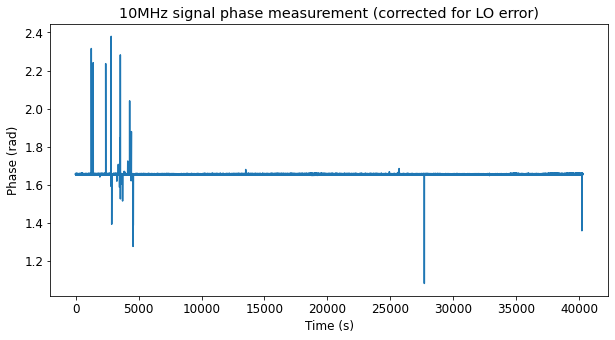
The measurements are post-processed in this Jupyter notebook. The first step in processing is to unwrap the phase measurement time series. Next, we need to compute and correct for the DDC local oscillator frequency error. In this case, the FGPA does round half-up as expected, so the frequency error is \(0.2\cdot76.8/2^{32}\) MHz, which is approximately 3.576 mHz. We generate the phase time series corresponding to this frequency \(f\) as \(\varphi(t) = 2\pi f t\) and add it to our unwrapped phase measurements. This corrects the local oscillator error.
The resulting phase measurements are plotted below. There are a few glitches which correspond to the the PLL being upset when there are samples filled with zeros due to lost packets. These glitches do not pose any problem for accurate frequency measurement. Since average frequency over an interval is computed as the difference quotient of phase over such an interval, we can just avoid choosing the glitches as endpoints of our measurement interval. It is not a problem if there are glitches inside the interval, because the PLL goes back to the correct phase after the glitch. Note that the PLL is very far from doing cycle slips, since the glitches are much smaller than \(\pi\) radians.
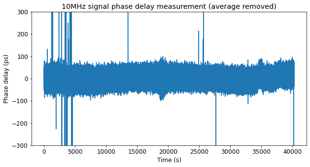
Dividing the phase by \(2\pi f_0\), where \(f_0\) is 10 MHz, we obtain the corresponding phase delay in seconds. We subtract the average delay, obtaining the next plot. Besides the glitches, we see that the measurement noise we get is on the order of 100 ps. This is due to thermal noise in the PLL.
In order to reduce the measurement noise, we could reduce the PLL bandwidth, or just average our measurements. By performing 100 second averages, we obtain the next plot. Now we can see that the delay varies a few tens of ps over the course of the measurement.
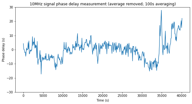
The cause of the delay changes is probably due to temperature dependence of the electronics. The measurement was done overnight, so the sudden change at 35000 seconds might correspond to the heating turning on in the morning. Since the 10 MHz signal is being radiated into the receiver rather than being conducted through a coax cable, in principle any change in the environment could also cause small changes in the phase delay.
Since this test was intended as a validation of the ability of measuring frequency accurately with the Hermes-Lite 2, these small delay changes are a mere curiosity. A similar experiment under more controlled conditions could be set up to measure the delay stability of the Hermes-Lite 2.
Note that the fact that after correcting for the DDC local oscillator error we have obtained a phase time series that is essentially constant over time means that we able to measure the 10 MHz from the GPSDO exactly. There are no frequency errors in the system, for otherwise we would see a linear slope in our phase measurements. (To be more precise, with our test we have only shown that any possible frequency error in the setup is less than some 50 ps over 40000 seconds, but this gives a frequency error on the order of \(10^{-15}\) parts per one, or 10 nHz when measuring 10 MHz. This frequency error is ridiculously small and wouldn’t affect in any practical application).
It is also interesting to compute the Allan deviation of our phase measurements. Note that however this doesn’t serve to validate that there aren’t frequency errors, since the Allan deviation is insensitive to constant frequency errors. To compute the Allan deviation, we use the method of overlapping intervals. The result is shown below.
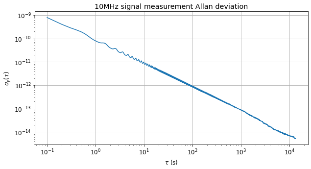
We see that the Allan deviation is essentially \(10^{-10}/\tau\). Our phase measurements are a white phase noise process, due to the PLL thermal noise, and there aren’t any other effects, so the Allan deviation should be \(C/\tau\), where the constant \(C\) is related to the white phase noise variance.
Hello Daniel,
thank you for the interesting article.
From the plot of σ_y(τ) I read σ_y(1 s) ≈ 10⁻¹⁰, so I would expect
σ_y(τ) ≈ 10⁻¹⁰/τ.
Best regards,
Roland
Thanks for spotting this! I have just fixed the mistake.