A few days ago, Emirates Mars Mission (Hope), and Tianwen-1 performed their Mars orbit injection burn (MOI). AMSAT-DL made a livestream for each of the two events, showing the X-band signals of the spacecraft as received with the 20m antenna at Bochum.
In the case of Tianwen-1 the signal was pretty strong even while the spacecraft was on the low gain antenna, and we could clearly see the change in Doppler rate as the thrusters fired up. However, in the case of Emirates Mars Mission the signal disappeared as soon as the spacecraft switched to the low gain antenna. In fact DSN Now reported a received power of -155 dBm with the 34m DSS55. That was a large drop from the -118 dBm that it was reporting with the high gain antenna. Therefore, nothing could be seen in the livestream waterfall until the spacecraft returned to the high gain antenna, well after the manoeuvre was finished.
Nevertheless, a weak trace of the carrier was still present in the livestream audio, and it could be seen by appropriate FFT processing, for example with inspectrum. I put up a couple of tweets showing this, but at the moment I wasn’t completely sure if what I was seeing was the spacecraft’s signal or some interference. After the livestream ended, I’ve been able to analyse the audio more carefully and realize that not only this weak signal was in fact the Hope probe, but that the start of the burn was recorded in perfect conditions.
In this post I’ll show how to process the livestream audio to clearly show the change in drift rate at the start of the burn and measure the acceleration of the spacecraft.
The idea with this post is that anyone can reproduce what I’m going to show. After all, the only data I’m using is the audio of a livestream that is recorded in Youtube. For convenience, I include with my code the segment of data I’m using, which is a 5 minute segment that starts 7850 seconds into the audio of the full video. If you want to start from scratch, you can use any webpage or application to download the audio of the full video, and work with that. In my case I used a webpage to download the audio in 320kbps MP3 format, then converted it to an 8ksps WAV file, and used SciPy to read the WAV file and extract the 5 minute segment.
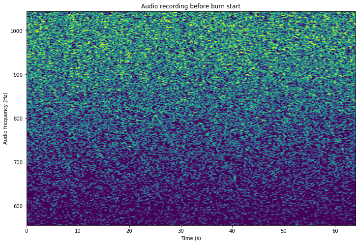
In the figure below you can see the waterfall of the first minute of the 5 minute clip I cut. The spacecraft signal can be seen as faint diagonal lines between 700 and 800 Hz. They are quite weak and have some fading, but hopefully you can see them.
There is something that is convenient to remark about the Doppler correction system that was used at Bochum for the livestreams. First, the system used the trajectory of the the spacecraft, ignoring the burn, to compute the expected Doppler. Therefore, the expected Doppler computation would be quite good before the burn started, but as soon as the thrusters fired it would diverge more and more from reality.
Second, rather than constantly adjusting the tuning to correct for Doppler and keep the signal exactly centred, the system performed discrete jumps of fixed size with the goal of keeping the signal inside a certain band, roughly 350 Hz wide. This had the effect of creating a sawtooth wave in the waterfall and the audio. As the signal arrived to one edge of this imaginary band, the Doppler correction performed a frequency jump to put the signal at the other edge of the band.
This can be seen quite clearly in the livestream of Tianwen-1. At the beginning of the livestream, the drift rate was quite low, since the spacecraft was well away from periapsis. Therefore, the period of the sawtooth was long. As the spacecraft approached periapsis and the drift rate increased, the period of the sawtooth kept reducing until it was quite short right before the burn. However, note that the amplitude of the sawtooth (this is, the width of this imaginary frequency band) is always the same.
The next figure shows the waterfall of the audio when the burn starts. It is a bit difficult to see, but hopefully you’ll be able to see two or three lines at the left around 800 Hz, and then a couple of lines going up in steps and with less slope, near the middle of the image.
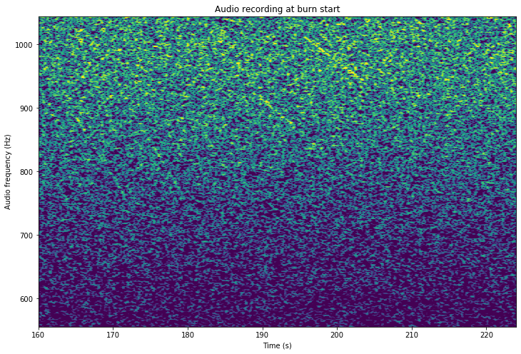
When the burn starts, the drift rate increases (i.e., changes from negative to less negative), since the retrograde burn accelerated the spacecraft towards Earth. As the Doppler correction keeps tuning in steps to correct for a more negative drift rate, we get steps upwards. This is the same that happened at the start of the burn of Tianwen-1. In that case the drift rate became almost zero, and then positive, since the thrust-to-mass ratio of Tianwen-1 is higher than that of Hope.
The resolution of the plots shown above, and those that come later is 0.98 Hz per FFT bin (FFT size of 8192 with a sample rate of 8ksps) and 64ms per time step (due to the use of overlapping FFT, and an advance of 512 samples per FFT).
In what follows, the idea is to undo the Doppler correction done at Bochum to join back the pieces of the sawtooth wave and also correct for the drift rate in order to get a signal of constant frequency that we may see clearly in a spectrum plot. To do this, we just need to create a sawtooth that has the same (or almost the same) phase, amplitude and period as the one that the Doppler correction created, and then use that sawtooth to control the frequency of a local oscillator with which we mix the audio signal. I have adjusted the parameters of the sawtooth by hand until I obtained something where the resulting signal before the start of the burn had a constant frequency and had no (or very brief) jumps.
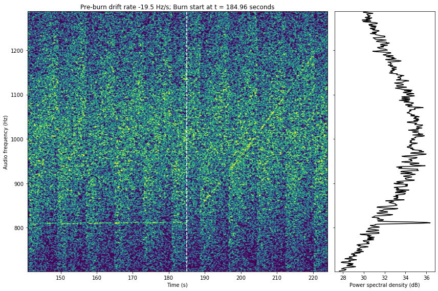
The result of this correction can be seen below. We see the signal before the burn as a flat line at constant frequency, slightly above 800 Hz, and then the signal rising up as the burn starts. The vertical white line marks the moment in which the start of the burn happens, which is at 184.96 seconds into this 5 minute segment. The right panel contains the spectrum plot of the data in the left of the waterfall (to the left of the white line). The signal can be seen very clearly, with an (S+N)/N of about 5dB, which would give an estimated CN0 on the order of 3 dBHz.
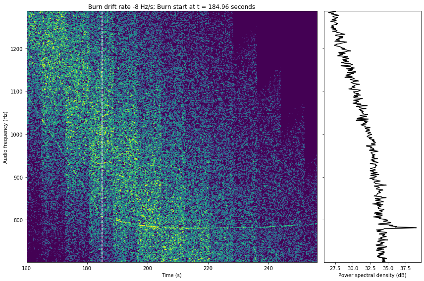
If we now change the drift rate correction, we can make flat the signal after the burn. We see that the drift rate is not constant, but rather it increases slightly with time, so it is not possible to find a drift rate that makes the line totally flat. I have chosen a drift rate that makes the line flat at approximately 20 seconds after the start of the burn. The right panel shows the spectrum of the right part of the waterfall (after the white line). Again, we have some 5 dB of (S+N)/N.
We have seen how by correcting the drift rate the “corner” of the Doppler curve, which marks the exact moment in which the thrusters started firing, can seen in the waterfall, whereas with the waterfall of the original audio signal it was impossible to see this corner. The moment in which the corner happens corresponds to 2:13:54.96 into the video, which by looking at the timestamps that appear in the screen shown in the video we can associate with 15:41:38 UTC (with a precision of perhaps one or two seconds). Since the light-time delay for this burn was 637 seconds, this means that the burn started at 15:31:01 UTC. This matches the official report of a start at 15:30 UTC, because it is possible that ullage motors fired one minute before the main burn, as we saw in Tianwen-1’s TCM-1.
The drift rate before the burn is -19.5 Hz/s, and when the burn starts it changes to -8 Hz/s. Such a drift rate change gives a line-of-sight acceleration of -0.41 m/s². This is just the projection of the acceleration vector onto the line-of-sight. In order to compute the full acceleration, we assume that it happened along the velocity vector of the spacecraft (with respect to Mars), and compute the projection of the unit velocity vector and the unit line-of-sight vector to Earth at the start of the burn. This computation ignores light-time delays, but is good enough for our purposes, since the line-of-sight vector changes slowly enough. The projection is 0.86.
This means that we only see 86% of the total acceleration in the Doppler drift rate. Therefore, the total acceleration must have been around -0.48 m/s². This contrasts to the theoretical acceleration of -0.58 m/s² that 720 N of thrust (since the spacecraft has 6x 120 N thrusters) applied to 1250 kg of mass produce (here the mass comes from a dry mass of 550 kg and 700 kg of fuel, assuming that the probe already spent in mid-course corrections 100 kg of its initial 800 kg).
Working backwards, we see that the measured acceleration of -0.48 m/s² would correspond to a thrust of 594 N. In fact, while I worked out the planning of the manoeuvre on Twitter, I noticed that the publicly stated burn length of 27 minutes was way too long to achieve the target orbit with a thrust of 720 N. To have a burn of 27 minutes that gave me the required apoapsis altitude I had to use a thrust of 658 N.
Note that all these calculations about the acceleration are just estimates, since we don’t know exactly the mass of the spacecraft, and our estimate of 1250 kg could be wrong by up to 10%. In any case, I think it is always good to go through these calculations to show what can be achieved with simple Doppler measurements and to check that the signal we observed matches what we expected.
The calculations and plots in this post have been done in this Jupyter notebook. The data file with the 5 minute segment of the livestream audio is included in the same repository. The results that I have shown are intended to be easily reproducible. It is possible to run the notebook with the supplied data or to start from scratch by downloading the audio from the livestream video on Youtube.
Many thanks and great work to all the AMSAT-DL team for organizing the livestreams. These were quite popular and were fantastic for outreach, as a wide audience could gather around a spectrum display and ask questions about spacecraft operations and communications via the livestream chat.
Fascinating! And congratulations to all involved in the capture & streaming of these signals.
I found your last point about the amount of thrust used for the orbit injection burn to be particularly interesting. That value for the thrust actually used (594 N) is VERY close to what would be possible if only 5 of the 6 thrusters were operated at 100% capacity.
Would it be reasonable to think that perhaps this value was chosen so that the mission would not be lost if one of the thrusters was determined to be defective at some point between Earth & Mars?
Hi Scott, I also noticed that, but perhaps it’s just a coincidence, since my estimate for the mass of the spacecraft (which is used in the thrust calculation) can have some error. So I can say that from the data we have it’s possible, but not sure, that the manoeuvre was done with only 5 thrusters instead of 6.
Why do you think the Doppler curve wasn’t flat during the burn? The loss of propellant mass is an obvious one, but I wonder if the thrust also varied during the burn due to thruster heating or propellant pressure variations. There were noticeable (but small) oscillations in spacecraft attitude during the burn as seen the video released by China TV.
I’m not sure. On the one hand I only corrected for a constant Hz/s term, and there are going to be higher order (Hz/s^2, etc.) terms due to the centripetal force changing direction and magnitude as the spacecraft moves closer to periapsis. However, before the burn these effects were small (I could make the curve seemingly flat over a scale of 30 seconds), so I guess that this is not the cause.
Then the reason must be that the acceleration from the propulsion is increasing, rather than constant. As you say, the decrease in mass (assuming constant thrust) already does that. However, I think that the mass flow rate is too small to cause the effect that we see. In fact -m'(t)/m(t) is on the order of 2e-4 1/s at the start of the burn, so we wouldn’t see any effects due to mass decrease over a scale of 60 seconds.
So it seems to me that the cause for the change in acceleration must be a change in thrust. I don’t know much about these thrusters (they are hydrazine thrusters), so I can’t say if the reason is heating, change in pressure, or something else.