As you may well know, DSLWP-B, the Chinese lunar orbiting Amateur satellite crashed with the Moon on July 31 as a way to end its mission without leaving debris in orbit. I made a post with my prediction, which showed the impact point southeast of Mare Moscoviense, in the far side of the Moon. Phil Stooke was more precise and located the impact point near the Van Gent crater.
Our plan is to get in contact with the LRO team and try to find the crash site in future LRO images. We are confident that this can be done, since they were able to locate the Beresheet impact site a few months ago. However, to help in the search we need to compute the location of the impact point as accurately as possible, and also come up with some estimate of the error to define a search area where we are likely to find the crash. This post is a detailed account of my calculations.
Digital Elevation Model
So far, all my estimates about the location of the DSLWP-B crash site had used a spherical model for the Moon, simply by asking GMAT to stop the simulation when the spacecraft’s altitude is zero. Phil Stooke recommended us to use a DEM (Digital Elevation Model) of the lunar surface. Since the lunar terrain is quite rough in comparison with Earth’s (changes of several kilometres in terrain height are pretty common all around the lunar surface), the impact site might change noticeably depending on the terrain.
Cees Bassa made a first try at using a DEM a few days ago. His results can be seen in this Jupyter notebook. They show that the impact point is inside the Van Gent X crater, several kilometres away from the location that would have been obtained by assuming a flat surface. This highlights the importance of using a DEM.
The spacecraft track that Cees used for his study is a CSV file published by Wei Mingchuan BG2BHC . The file can be found here. It describes the trajectory of the spacecraft in latitude, longitude and altitude coordinates. The problem with this CSV file is that we are not sure about which hypotheses were used to generate it.
The Moon is much more round than Earth, owing to its low rotational speed. It has an equatorial radius of 1738.1km and a polar radius of 1736.0km. Therefore, for many purposes a spherical model instead of an ellipsoidal model is used. However, there is not a standard lunar radius for the spherical model, and values differing up to 1km are used.
There are two ways of using latitude and longitude coordinates. The first is the geocentric coordinates (called planetocentric coordinates for bodies other than the Earth). These are the well known spherical coordinates. The second is the geodetic coordinates (called planetodetic coordinates for bodies other than the Earth). These use a reference ellipsoid and take into account the ellipsoid flatness, as seen in these formulas. The geocentric coordinates are a special case of geodetic coordinates, where the reference ellipsoid is taken to be a sphere.
For mapping the Earth surface, geodetic coordinates are used almost always. The difference between geodetic and geocentric coordinates is quite noticeable. In the case of the Moon, since its flatness is much smaller than Earth’s, it is common to use planetocentric coordinates instead of planetodetic. The difference between the two coordinates system is smaller than for Earth, but it may still be important for some applications.
The problem with the CSV file generated by Wei is that we don’t know if it uses planetocentric or planetodetic coordinates, nor which is the reference sphere or ellipsoid used to generate the coordinates. Another problem is that we are not sure about the accuracy of the orbital propagation model used to compute the spacecraft’s position in Wei’s file.
In order to have full control over all these parameters, I decided to use GMAT to propagate the orbit and generate the trajectory of the spacecraft in a completely known reference system.
The Digital Elevation Model that Cees is using is SLDEM2015. It is a global model with a resolution of approximately 60m and a vertical accuracy of 3 to 4m. It was generated with data from the Lunar Orbiter Laser Altimeter (LOLA) instrument on-board LRO and the terrain camera on-board the Japanese Kaguya (SELENE) orbiter. More information about this model can be found in this article.
The model can be downloaded here in 30×45 degree tiles. The tile that we use for the DSLWP-B crash site is sldem2015_512_00n_30n_135_180_float.img. Its description can be read here. From this description, it is clear that the file uses a spherical model for the Moon with a radius of 1737.4km. Therefore, the latitude and longitude coordinates used in the DEM are planetocentric.
Additionally, to define the body-fixed coordinate system, the DEM uses the mean Earth/polar axis of DE421, also called MOON_ME. By default, GMAT uses the DE405 solar system ephemeris, but it can be switched to DE421. However, in GMAT, the body-fixed coordinate system of the Moon is defined by the principal axis system, also called MOON_PA. It seems that it should be possible to change this to MOON_ME just by changing the Luna.SpiceFrameId paramter, but the software complains that this parameter cannot be changed in newer versions, and I can confirm that trying to change it makes no effect to the results.
Fortunately, the rotation between MOON_PA and MOON_ME is described by a constant matrix that appears in this document. According to the SPICELunaFrameKernel.tf file in GMAT, the rotation between MOON_PA and MOON_ME in DE421 represents a displacement of 875m on the lunar surface, so the difference is important when computing the DSLWP-B crash site.
In trying to obtain the best compatibility possible with the DEM, I use the DE421 ephemeris in GMAT and output a file with the spacecraft positions in cartesian lunar body-fixed coordinates using the MOON_PA frame. These positions are then rotated to MOON_ME in Python.
The crash.script GMAT script is used to propagate the spacecraft orbit and the demtrack.py Python file (which is intended to be imported from a Jupyter notebook) is used to load up the DEM, load the GMAT output file, convert from MOON_PA to MOON_ME coordinates, compute latitude, longitude and altitude assuming a lunar radius of 1737.4km, and compute and plot the impact point of the spacecraft’s track with the DEM surface.
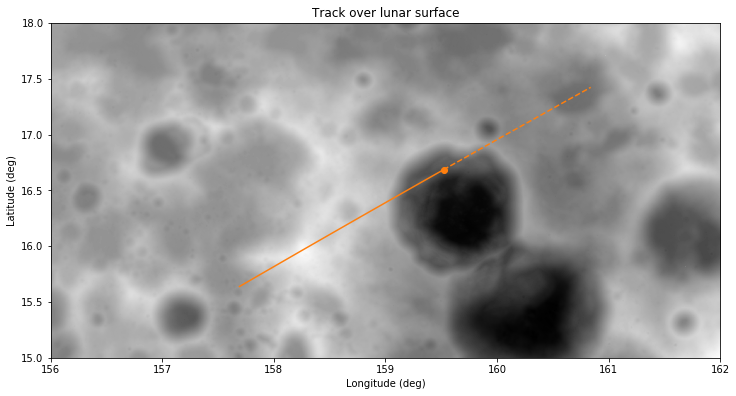
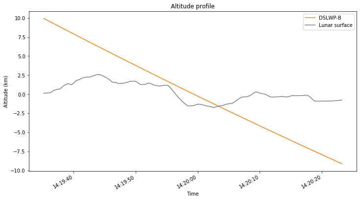
The calculations are run from this Jupyter notebook. The figure below shows a track generated with the ephemeris from July 25 that I used in my previous post. DSLWP-B passes approximately 500m above the western rim of Van Gent X crater, enters the crater, and impacts against its northern wall. At a first glance, the results looks close to those obtained by Cees Bassa.
Ephemerides and orbital models
The next step is understanding how much effect do different ephemerides and orbital propagators have on the location of the impact point. This serves to estimate the error of the crash site location prediction and define a search area.
The figures shown above have been done using the ephemeris from July 25 generated by the Chinese DSN. These are the best ephemeris I have so far, since Wei hasn’t been able to find some ephemeris for a later epoch yet.
The force model used in GMAT is rather accurate and it is what I have been using for most of the simulations throughout the mission. It considers the Moon non-spherical gravity using spherical harmonics up to degree and order 10 taken from the LP165P model, the point masses of all the other major bodies in the solar system, solar radiation pressure (although the area and reflectivity coefficients are very rough approximations), and relativistic corrections.
Therefore, in my opinion, the figure shown above represents a good estimate of the impact point, and I will use it as a reference to judge impact points generated using other methods. The coordinates of this reference point are the following:
Latitude 16.6858 deg, Longitude 159.5218 deg, Altitude -1561.12 m
As mentioned above, this assumes a spherical Moon with a radius of 1737.4km and uses the DE421 mean Earth/polar axis reference system.
The first test I have done, to have a coarse estimate of the error of the Chinese DSN ephemerides and the orbital model is to use older ephemerides. The impact point is computed with these older ephemerides and compared with the reference position in East, North, Up (ENU) coordinates. The results are as follows:
Ephemeris from 2019-07-18
East = -64.6 m, North = -221.6 m , Up = -93.1 m

Ephemeris from 2019-06-28
East = 490.5 m, North = -72.6 m , Up = -86.2 m
We see that the error obtained by using older ephemerides is only of several hundreds of metres, even if we use the ephemeris from 2019-06-28, which were taken more than one month before the impact.
Another important task is to compare these results with the CSV file generated by Wei and the results obtained by Cees. Cees gives the coordinates for the impact as latitude 16.675 deg, longitude 159.617deg. In the ENU system centred on my reference point, these are:
East = 2766.3 m, North = -326.9 m
There is a rather noticeable difference of approximately 3km between the result by Cees and the positions I have obtained. If I load up the CSV file made by Wei and study it using my code, I get an impact position of
East = 2752.9 m, North = -311.6 m , Up = -316.0 m
This differs from only in 20m from the position that Cees has obtained. Here we are using the same data for the spacecraft track and DEM, but are doing the calculations independently, using a different algorithm, which explains the difference in positions.
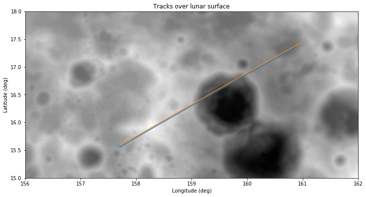
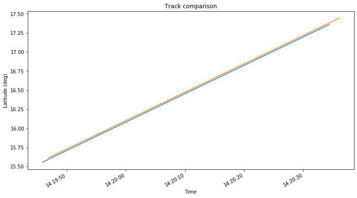
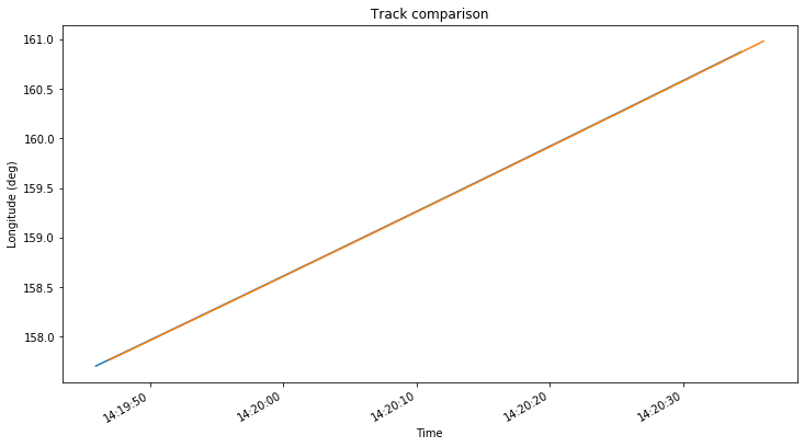
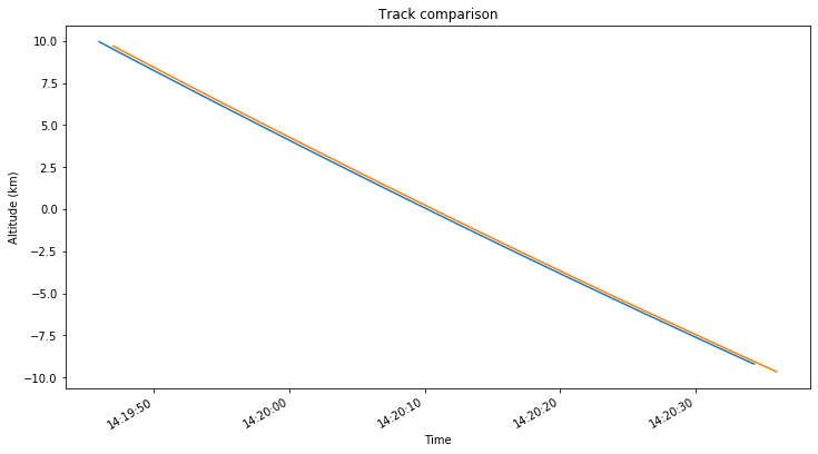
The difference between the positions obtained with Wei’s CSV file and my GMAT simulations is so large that it is worth investigating. The figures below show a comparison of the spacecraft tracks, with my GMAT simulation using the July 25 ephemeris in blue and Wei’s CSV in orange.
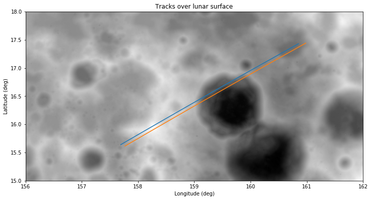
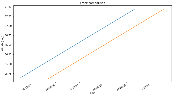
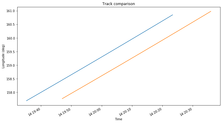
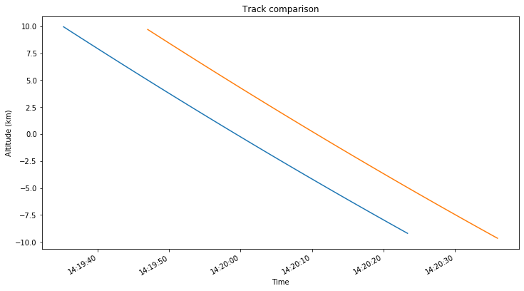
It seems that Wei’s track is displaced a few km to the southeast with respect to my track. This makes me suspect about the orbital model used by Wei to generate the CSV.
As a simple test, I run my GMAT simulation using point mass gravity for the Moon. The results are seen below in blue, with Wei’s track in orange. We see that the track generated with spherical gravity in GMAT is much closer to Wei’s track.
The impact point of this GMAT spherical gravity track is given in ENU coordinates as:
East = 3192.5 m, North = -752.4 m , Up = -548.5 m
This is 1150m away from the impact point computed with Wei’s CSV file. Part of this difference may be caused by the difference between the MOON_PA and MOON_ME reference frames. Indeed, if I skip the conversion from MOON_PA to MOON_ME when loading the GMAT spherical gravity track, I get an impact of
East = 3043.6 m, North = -504.8 m , Up = -431.3 m
which is only 870m away from the impact of Wei’s CSV file.
From talking about this problem with Wei, it seems that he is indeed using spherical gravity for the Moon, though I am not completely sure about it. He says he is using STK with the propagator Earth HPOP Default v10.
I think that it is important to use a good non-spherical gravity model for the Moon when computing the impact location, as we have seen that the prediction can change by more than 3km depending on the gravitational model used. Since DSLWP-B’s orbit is elliptical, the non-spherical gravity of the Moon perturbs the orbit noticeably as the satellite passes through the periapsis. Before the crash, the latest periapsis height was only 13km, so non-spherical gravity plays an important role.
Already going to a gravitation model with spherical harmonics of degree up to 2 and order 1 (i.e., considering only the Moon oblateness) gives a similar track to the one with 10×10 spherical harmonics and an impact point of
East = 619.8 m, North = 705.0 m , Up = 152.3 m
Therefore, it seems that most of the effect in the impact point due to the non-spherical gravity is caused by the oblateness term.
To assess whether a 10×10 gravity model is accurate enough for the calculation of the impact point, a simulation with a 20×20 model taken from LP165P has been done using the GMAT ephemeris. This gives an impact point coordinates of
East = 66.8 m, North = 31.8 m , Up = 1.2 m
Since the difference between the 10×10 and 20×20 gravity models is smaller than the error we expect to have in the ephemeris, we conclude that a 10×10 gravity model is appropriate.
Monte Carlo experiments
We do not know the accuracy of the July 25 ephemeris that we are using for the calculations. Often, a state error covariance matrix is used to describe the accuracy, but we don’t have such a matrix. Therefore, Cees suggested to see what would happen if we assumed a position error of 1km in the ephemeris.
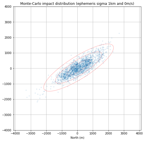
To answer Cees’s question, I have run a Monte Carlo simulation where the July 25 ephemeris (in cartesian state) are perturbed using a Gaussian error with a sigma of 1km in position and 0m/s in velocity. The impact point coordinates for each trial are then saved for later analysis. The calculations are done in this Jupyter notebook.
After generating more than 2000 impact points, I plot the results on top of the DEM map, as shown in the figure below.
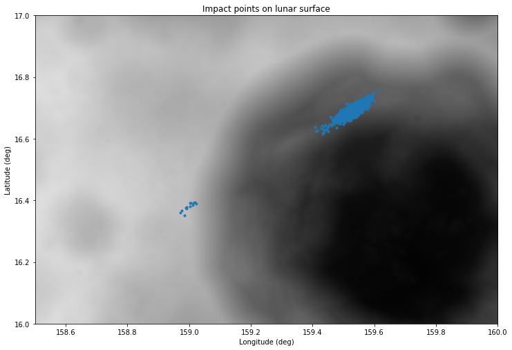
Most of the impact points are in an ellipsoidal area on the northern wall of Van Gent X. The area is more spread in the direction of DSLWP-B’s orbit, which makes sense. A few of the simulations haven’t managed to clear the western rim of Van Gent X and have impacted on the rim instead.
The points that impact outside of the crater are labeled as outliers and shown in orange in the figure below, which uses ENU coordinates with respect to the reference point given above.
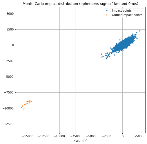
Only 0.6% of the impact points have been classified at outliers, so the probability that DSLWP-B crashed outside of Van Gent X is low.
The covariance of the non-outlier points is then computed in order to give an error ellipse. The eigenvalues of the covariance matrix, which indicate the semi-axes of the ellipse are 876 and 239m. The orientation of the major axis is 57.6º with respect to north.
The figure below shows the non-outlier points with the 1-sigma, 2-sigma, and 3-sigma ellipses.
It is not easy to judge whether the orbital error model of a 1km sigma in position is realistic or not. In my opinion the orbital error should be smaller, and the 1km sigma should be taken as a worst case scenario. Indeed, using the ephemeris of June 28, we obtained an impact point well inside the 1-sigma ellipse of the 1km sigma error model.
Comparison with radio observations
Another idea that Cees suggested to validate the ephemerides was to compare them with radio observations of the Amateur payload done on the days before the crash. One of the things that can be observed are radio occultation timings. According to GMAT with the July 25 ephemeris, the following radio occultations happened before the crash:
2019-07-26 11:31:22.793 --- 2019-07-26 12:15:56.704
2019-07-27 07:53:41.841 --- 2019-07-27 08:35:54.149
2019-07-28 04:17:37.714 --- 2019-07-28 04:56:15.064
2019-07-30 17:38:30.129 --- 2019-07-30 18:07:41.744 (see update)
2019-07-31 14:08:27.941 --- crash
From these occultations, only the ones on July 26 and July 31 were recorded in Dwingeloo. The IQ recordings can be found here.
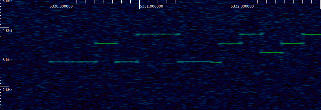
For July 26, the start of the occultation was observed both in the 435.4MHz and 436.4MHz frequencies at 2651.5 +/- 0.5 seconds since the beginning of the recording. This is a coarse timing for the occultation obtained by looking at the waterfall in inspectrum rather than a precise timing obtained by fitting a diffraction curve.
The end of the occultation was not observed on any of the frequencies. Cees twitted that the occultation ended during a JT4G transmission at 435.4MHz, but as it can be seen in the figure below, the first JT4G tone comes on cleanly rather than being diffracted. This means that the JT4G transmission started shortly after the occultation end.
The recording done on July 26 is timestamped with a start time of 10:47:03 UTC. This is only included in the filename, so I am not completely certain about the accuracy of this timestamp (see below). According to this timestamp, the occultation started at 11:31:14.5 UTC. This is 8.3 seconds before what predicted by the ephemeris.
For July 31, the start of the occultation was observed on both frequencies at 2775 +/- 0.5 seconds after the start of the recording. The recording of July 31 is in GNU Radio metadata format and includes timestamps taken from GPS. The timestamp at the beginning of the file is 2019-07-31 13:22:10.490141 UTC. Thus, the occultation started at 14:08:25.5 UTC. This is 2.4 seconds before what predicted by the ephemeris.
However, the filename says that the recording started at 13:22:02 UTC. Thus, it seems that the filename timestamp is wrong by 8.49 seconds. This perhaps explains the error of 8.3 seconds seen in the July 26 occultation. If we assume that the timestamp in the filename of the recording is 8.5 seconds earlier than the real start of the recording, then it turns out that the July 26 occultation started only 0.2 seconds after what predicted by the ephemeris.
To summarise, we have the following differences between the radio observations of the occultations and the July 25 ephemeris:
July 26:  0.2 +/- 0.5 or 8.3 +/- 0.5 seconds ?? (see update below)
July 31: -2.4 +/- 0.5 seconds
It is not easy to judge the accuracy of the ephemeris from these numbers. First of all, the usefulness of occultation timings is limited, since any difference between the observation and the ephemeris can be explained by a change in mean anomaly, so that the spacecraft travels the same track at a different time, and the change in the impact point location is very small. However, it is worthy to remark that the error in ocultation timings from these ephemeris are an order of magnitude smaller than those observed in my diffraction study, giving more confidence in the accuracy of the July 25 ephemeris.
Cees has also suggested to perform analysis to other parameters of the radio observations, such as the Doppler curve. I am not so sure about the usefulness of Doppler observations. On the one hand there is an unknown transmitter frequency offset, and on the other hand the Doppler usually changes rather slowly, so I am not sure how much can the orbital elements be constrained by Doppler observations.
Update 17:00 UTC: Cees says that he wouldn’t trust transferring the timestamp offset from the tagged recorded to the untagged recording, since these are done in a different computer. He has also noticed that I have forgotten to process two occultations: the one on July 28 (probably because I didn’t see the corresponding recording made at Dwingeloo), and the one on July 30 (because it wasn’t originally listed in the GMAT output, as it happened below 7 degrees of elevation).
I have now processed the occultations on July 28 and July 30. The observation results are as follows:
July 28:
Entry: 04:17:38.3    Exit: 04:56:15.3
July 30:
Entry: 17:38:28.9    Exit: 18:07:41.9
Thus, we obtain the following differences between the observations and GMAT simulation.
July 26 (entry):  0.2 +/- 0.5 or 8.3 +/- 0.5 seconds
July 28 (entry):  0.6 +/- 0.5 seconds
July 28 (exit):   0.2 +/- 0.5 seconds
July 30 (entry): -1.2 +/- 0.5 seconds
July 30 (exit):   0.2 +/- 0.5 seconds
July 31 (entry): -2.4 +/- 0.5 seconds
LRO imaging
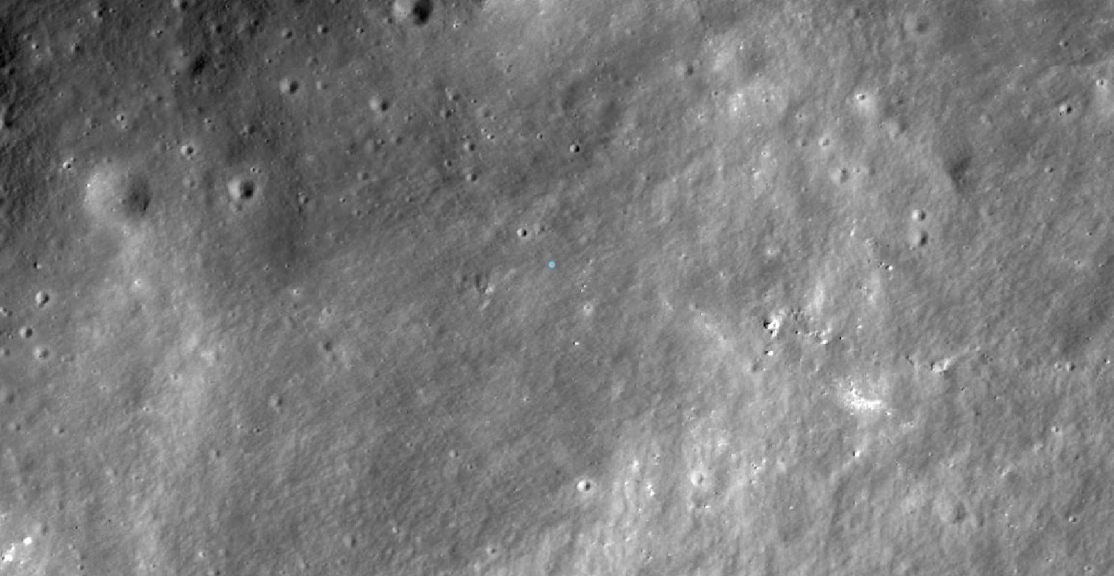
According to the calculations above, I expect that the impact point of DSLWP-B should be located near the reference position given by the following planetocentric coordinates in mean Earth/polar axis:
Latitude 16.6858 deg, Longitude 159.5218 deg
I estimate an error of perhaps 600m in the northeast direction and 200m in the southeast direction. This area can be seen here in Quickmap, with the reference point marked (also shown in the figure below for convenience). Fortunately, it seems that the area has few craters, so perhaps it is not difficult to observe any alterations to the terrain.
LRO has three cameras: the wide angle camera (WAC), and two narrow angle cameras (NAC). The NACs have a resolution of 0.5 metres and a swath of 5km. Since LRO is in a polar orbit, NAC images are strips which are 5km wide in the east-west direction and many kilometres long in the north-south direction.
According to the calculations above, it seems enough to take a single NAC image over the reference position in order to have confidence that the real DSLWP-B crash site will appear in the image. To cover a wider area, two or three adjacent NAC images may be taken.
Quickmap can also search for NAC images that contain our reference point. The results are shown here. We see that there are four NAC images available. These can be explored individually, but the interface is not so easy to use as Quickmap, and the east-west directions are swapped. I have taken a look at image M1107231635RC and found that the reference position is around line 8500, sample 3364.
Wonderful write-up! Just fascinating.
Do we have any information regarding how often the LRO images a given spot? Or better yet, when we might expect the target area to be imaged again assuming no deviation to the normal routine of the LRO?
Thanks!
Hi Scott,
I’m not an expert on LRO’s mission, but I can give you some answers. First of all, LRO is in a polar orbit, so it travels along the lunar surface from north to south or viceversa. To image an area, LRO needs to pass over that area. Half of the orbit is in daylight and half is in darkness, so only the illuminated half of the orbit can be used to take images.
To image a particular area, you need to wait until the orbit passes over that area. This happens because the Moon rotates under the orbit. The Moon does a full rotation every lunar month (27 days). So LRO revisits the same area every 27 days.
Finally, LRO doesn’t spend all its time taking images. That would be a really incredible amount of data to send back to Earth. This is the reason why there are only 4 images of the crash site area in the archives, even though LRO has passed over this area hundreds of times.
Only areas of particular interest (scientific targets) are imaged again. This is the reason why we intend to contact the LRO team, so that they can command the spacecraft to take an image when it passes over Van Gent X.