During my research and experiments about using WSJT-X modes through linear transponder satellites, one of the questions I had is by how much do TLEs of different epochs for the same satellite vary. This was glimpsed in part II, where I plotted the “best delay” parameter for TLEs of different age.
The topic of accuracy in TLE computation and propagation is rather complex. A NORAD TLE is the result of an orbit determination after several radar measurements at different epochs, so the elements are in some sense “averaged” over time. Also, the SGP4 propagator is simple and doesn’t model many orbit perturbations. However, NORAD TLEs are specially crafted to give improved results when used with SGP4.
Nevertheless, here I present a simple way of studying the rate of change of NORAD TLEs at different epochs. This procedure might not be very meaningful or sophisticate, but still seems to yield some interesting results.
The main idea in this study is to define a metric that measures the “variation” between consecutive TLEs for the same object. The metric I’ve chosen is rather naïve. Given two TLEs \(T_1\) and \(T_2\) (where \(T_1\) is older than \(T_2\)), we define the variation from \(T_1\) to \(T_2\) as the distance between the position of the object at the epoch of \(T_2\) predicted with \(T_1\) and the position of the object at the epoch of \(T_2\) predicted with \(T_2\), divided over the difference of the epochs of \(T_2\) and \(T_1\). Thus, the TLE variation has units of m/s.
I have used Python to download from Space-Track all the TLEs for several active Amateur satellites generated during the year 2017. Thus, I am studying all TLE data for almost a year and a dozen of objects. I haven’t found a completely satisfactory way of plotting the results. The best I’ve been able to come up with is to do semilog plots of the TLE variation, organized by families of satellites. The results are below.
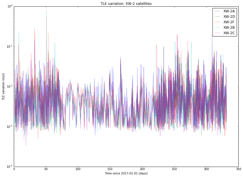
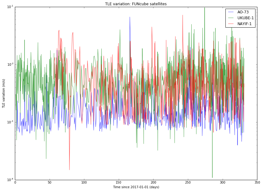

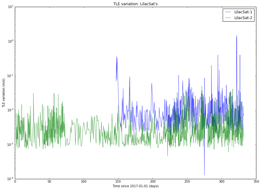
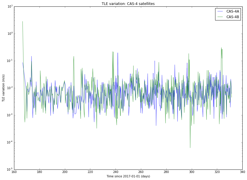
We note that the TLE variation changes erratically between approximately \(10^{-3}\) and \(10^{-2}\)m/s. This is is an order of magnitude, so in principle it is difficult to predict TLE variation accurately. It is also noteworthy that the variation for SO-50 is much more steady than for the other satellites. I find this very curious and I don’t have any explanation for this effect. Also, we note that there are some satellites such as AO-7 and FO-29 whose TLEs vary more slowly than the TLEs of newer, lower orbiting satellites.
The TLE variation can be related to the “best delay” parameter introduced in previous posts. Assuming an orbital speed of 7800m/s, which is typical for a LEO satellite, and assuming that all the variation happens in the along-track direction, a variation of \(10^{-2}\)m/s corresponds to a delay \(\delta\) of 0.11s per day. This matches the studies I have done with LilacSat-1 in previous posts. It also means that FT8 can be used with TLEs which are 1 or 2 days old without the need to perform a search in \(\delta\).
I have also done another study with the same TLE data. For each object, I pick all pairs \((T_1, T_2)\) of TLEs and compute the same distance as above (the distance between the predictions at the epoch of \(T_2\) according to \(T_1\) and according to \(T_2\)). Then, I plot these distances with respect to the difference between the epochs of \(T_2\) and \(T_1\). This gives an estimate of the error in prediction (in meters) according to the TLE age (in days). A loglog plot seems to work best. The results are shown below.

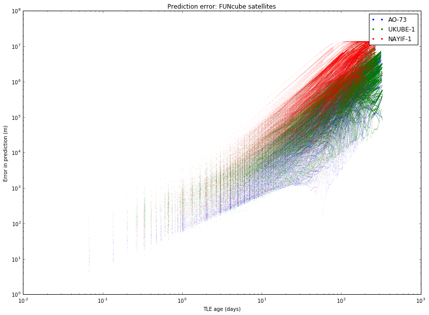
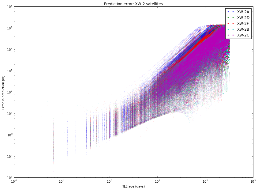
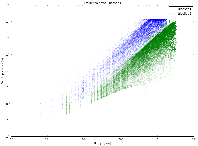
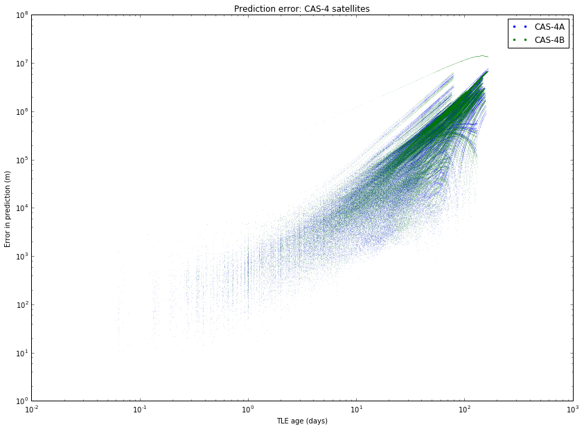
We note mainly two things. First, that different satellites have different degrees of “stability” in their TLEs. This was also observed in the graphs of TLE variation. Second, the slope of the cloud of points seems to change at around 10 days.
The most interesting case to study is between 1 and 10 days, since it is unusual to use TLEs older than 10 days, as the error is too large. It seems that for an age between 1 and 10 days all the clouds of points have the same slope, suggesting that we can model the error as \(E(t) = C_s t^\gamma\), where \(t\) is the \(t\) TLE age, \(\gamma\) is a fixed constant, and \(C_s\) is a constant depending on the satellite. To estimate \(\gamma\), we collect all the clouds of points between 1 and 10 days and do a least squares fit.
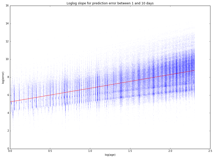
The slope of the least squares fit is 1.5276, so its seems that taking \(\gamma = 3/2\) is a good approximation. Note that this means that the prediction error doesn’t grow linearly with the TLE age, but rather as the TLE age to the power \(\gamma\).
As a final remark, a rule of thumb is that the accuracy of NORAD TLEs is around 1km at the epoch and degrades 1 or 2km per day (see here). My results seem to follow more or less this rule of thumb. Some interesting articles about the accuracy of TLEs are Validation of SGP4 and IS-GPS-200D Against GPS Precision Ephemerides by T.S. Kelso and Accuracy Assessment of SGP4 Orbit Information Conversion into Osculating Elements by S. Aida and M. Kirschner. I still need to find some time to read them in detail.
The computations for this post have been carried out in this Jupyter notebook. One of the useful things in this notebook is the code to download and parse the TLEs from Space-Track automatically.
Great work
Amazing, I need a quite weekend to try and understand your research.