DME (distance measuring equipment) is an aircraft radio navigation system that is used to measure the distance between an aircraft and a DME station on ground. DME is often colocated with a VOR station, in which case the VOR provides the bearing information. DME works by measuring the two-way time of flight of pulse pairs, which are first transmitted by the aircraft, then retransmitted with a fixed delay by the ground station, which acts as a transponder, and finally received back by the aircraft. DME operates between 960 and 1215 MHz. It is channelized in steps of 1 MHz, and the air-to-ground and ground-to-air frequencies always differ by 63 MHz (here is a list of all the frequency channels).
I want to write a post explaining in detail how DME works by analysing a recording of DME that contains both the air-to-ground and the ground-to-air channels. Among other things, I want to show that the delay between the aircraft and ground station pulses matches the one calculated using the aircraft position (which I can get from ADS-B data on the internet), the ground station position, the position of the recorder, and the fixed delay applied by the ground station transponder.
Recording two channels 63 MHz apart is tricky with the kind of SDRs I have. Devices based on the AD9361 technically support a maximum sample rate of 61.44 Msps (although some people are running it at up to 122.88 Msps). The LMS7002M, which is used by the LimeSDR and other SDRs, is an interesting alternative, for two reasons. First, it supports more than 61.44 Msps. However, it isn’t clear what is the maximum sample rate supported by the LimeSDR. Some sources, including the LimeSDR webpage mention 61.44 MHz bandwidth, but the LMS7002M datasheet says that the maximum RF modulation bandwidth (whatever that means) through the digital interface in SISO mode is 96 MHz. In the case of the LimeSDR there is also the limitation of the USB3 data rate, but this should not be a problem if we use only 1 RX channel. I haven’t found clear information about the limitations of each of the components of the LMS7002M (ADC max sample rate, etc.).
The second interesting feature is that the LMS7002M has a DDC on the chip. The AD9361 has a series of decimating filters to reduce the ADC sample rate and deliver a lower sample rate through the digital interface. The LMS7002M, in addition to this, has an NCO and digital mixer that can be be used to apply a frequency shift to the ADC IQ signal before decimation.
I had two different ideas about how to use the LimeSDR to record the two DME channels. The first idea consisted in using a 70 Msps output sample rate. For this I used an ADC sample rate of 140 Msps, because I think it is necessary to have at least decimation by 2 after the ADC (the LMS7200M documentation does not explain this clearly, so figuring out how to use the chip often involves some trial and error using LimeSuiteGUI). This idea had two problems. The first problem is that some CGEN PLL occasionally failed to lock when using an ADC sample rate of 140 Msps. However the LimeSuite driver retried multiple times until the PLL locked, so in practice this wasn’t a problem. This approach worked well on my desktop PC, since in 70 Msps I had the two DME channels and then I could use GNU Radio to extract each of the two channels (for instance with the Frequency Xlating FIR Filter). However, the laptop I planned to use to record on the field couldn’t keep up with 70 Msps.
The second idea was to use the on-chip DDC in the LMS7200M to extract the DME channel and deliver a much lower sample rate over the digital interface. The figure below shows how the LMS7200M digital signal processing datapath works. This datapath is called RXTSP. The RXI and RXQ signals are the digital signals coming from the ADC (here and below, by ADC I mean a dual-channel ADC, since the LMS7002M is a zero-if IQ transceiver). The RYI and RYQ are the signals delivered to the digital interface of the chip. Since the LMS7200M has two RX channels, there are two identical chains, one for each channel. The parameters of each chain can be programmed completely independently.
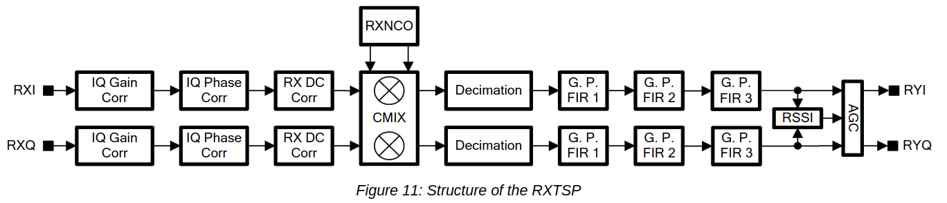
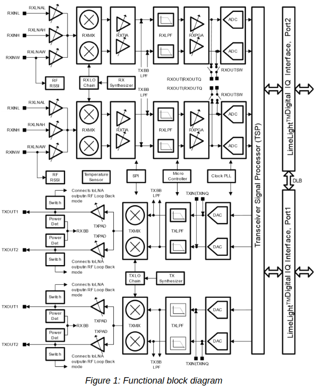
There is no way of sending the signal of one ADC to the two RXTSPs. The connection between each ADC and its corresponding RXTSP is fixed. Therefore, we need to feed in the antenna signal through the two RX channels, but we can easily do this with an external splitter. Remember that both of the LMS7200M RX channels share the same LO, as illustrated by the block diagram below. So the point here is to tune the LO to a frequency between the two DME channels, set the sample rate high enough that both DME channels are present in the ADC output, and finally to use each of the two RXTSPs to extract one of the DME channels, sending it at a low sample rate through the digital interface.
This approach has worked quite well. I have set the ADC to 80 Msps and used the RXTSPs to dowconvert and decimate the DME channels to 2.5 Msps, recording that data directly in GNU Radio.
I have done a two hour recording of DME and published it in the Zenodo dataset Recording of Colmenar (CNR) VOR-DME air-to-ground and ground-to-air DME channels.
In the rest of this post I explain the details of the recording set up and do a preliminary analysis of the recording quality.
VOR-DME and recording location
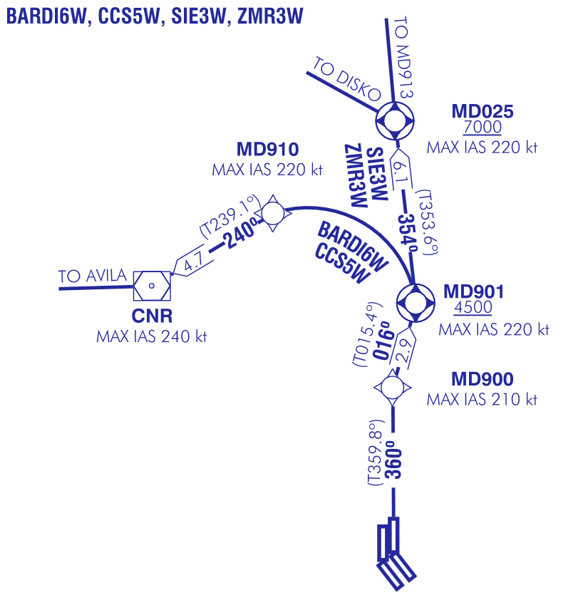
The VOR-DME station used in this recording is the Colmenar (CNR) VOR-DME, which is the one closest to where I live. The VOR has a frequency of 117.3 MHz. The DME frequency is related to the VOR frequency, so according to the list, it corresponds to TACAN channel 120X, which has an aircraft-to-ground frequency of 1144 MHz and a ground-to-aircraft frequency of 1207 MHz (DME is, in a sense, a civilian version of the military TACAN radio navigation system, which provides both range and bearing information).
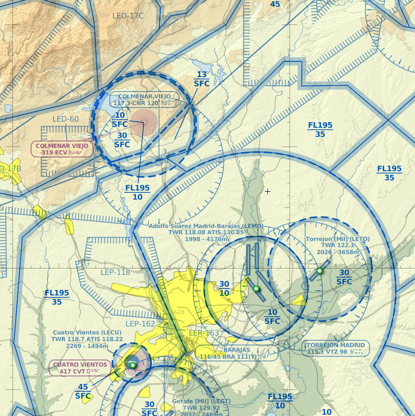
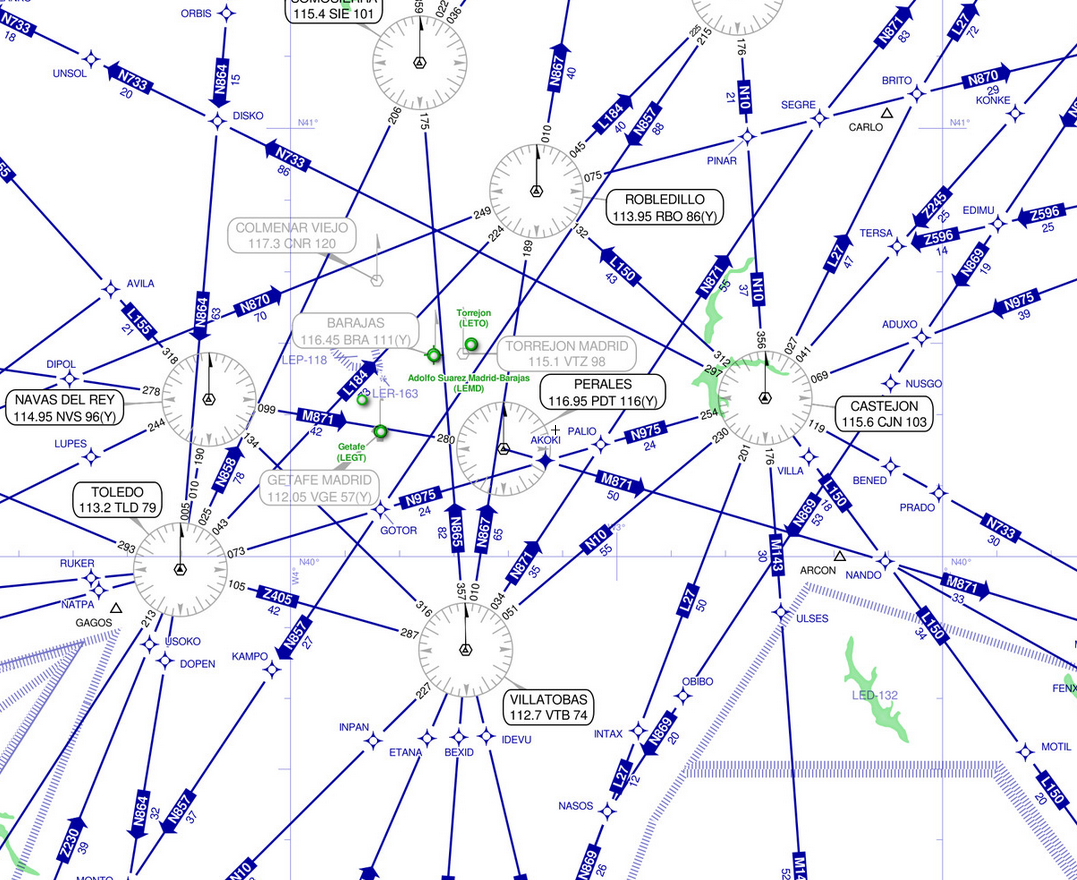
According to the Skyvector world high and world low IFR maps, the CNR VOR is not part of any airway. However, it is part of several instrument procedures of the Madrid Barajas airport. An aircraft only transmits to a DME station if that DME or VOR-DME station is selected in one of the aircraft navigation radios (most aircraft have two radios for VOR-DME). The pilot will usually tune the radios to the stations that are part of the procedure that the aircraft is flying (although the pilot is free to tune to other stations as a cross check), so the kind of aircraft that we expect to see in the recording are those operating on the Madrid Barajas airport, not those flying high en route.
In particular, aircraft departing from Madrid Barajas runway 36R and flying due west or southwest will fly over CNR.
However, departures from runway 36L do not use the CNR VOR at all (see the SID chart). I’m quite impressed at how much the instrument procedures for Madrid Barajas have changed since I did my 2.3 GHz aircraft reflections recording in 2018. This is due to the increasing prevalence of GPS navigation.
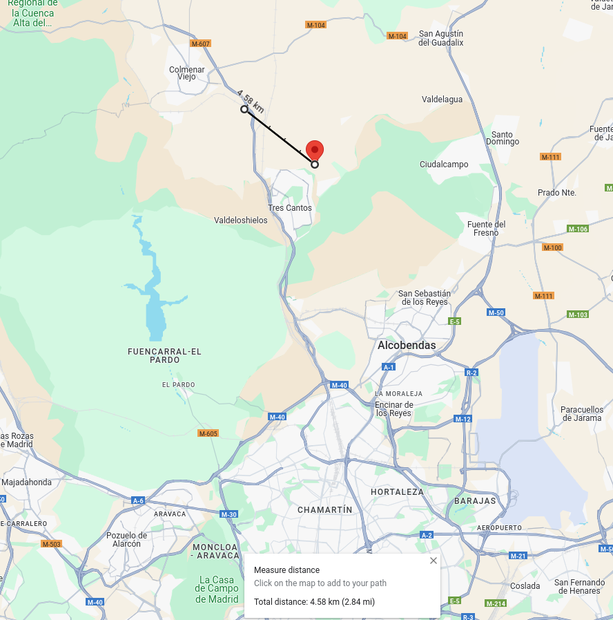
The location I have chosen to do the recording is in the countryside just outside my town. It is 4.58 km southeast of the CNR VOR-DME. There is almost line of sight to the VOR-DME station, but there are some buildings in between. This recording location also gives good geometry for TDOA (time difference of arrival) analysis for aircraft travelling along the path shown above. As they depart from Madrid Barajas, they are closer to my recorder than to the VOR-DME, but at some point they start being closer to the VOR-DME than to my recorder.
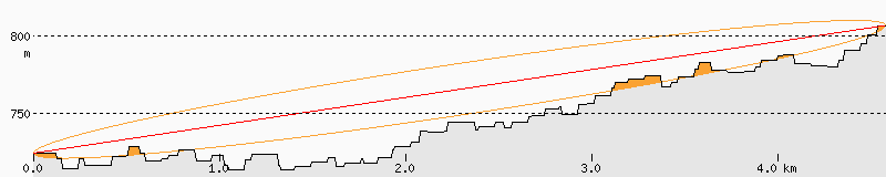
The HeyWhatsThat profile shows that there are no significant terrain obstructions.
Antenna
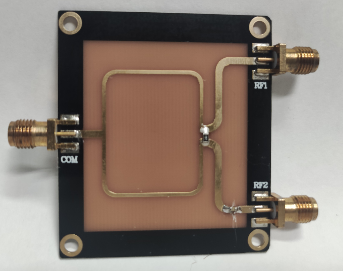
I have made an antenna from scratch for this recording. I have chosen a quarter-wave groundplane monopole because it’s easy to make and gives a roughly omnidirectional pattern, except for a null in the zenith (which is useful, because I’ll be recording both the ground signal and signals from aircraft at high elevation angles). I made the antenna from a spare SMA female connector and some thick enamelled copper wire.
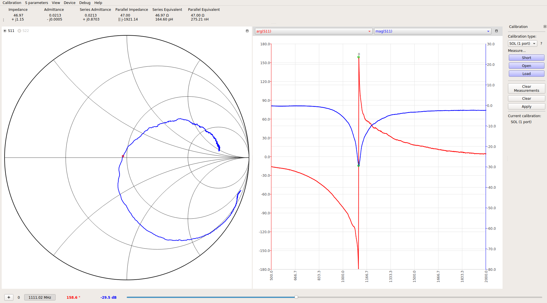
The following photo shows the antenna and the LNA, with a ruler in cm for scale.
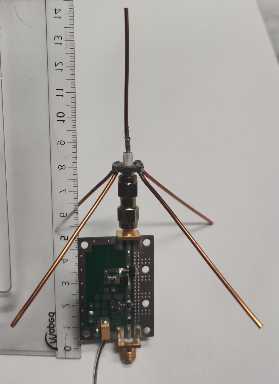
The antenna is resonant somewhere around 1.1 to 1.2 GHz, depending on the presence of nearby objects. It provides a good impedance match to 50Ω in all the DME band.
LNA
Since the antenna will be connected to the two RX channels of the LimeSDR through a splitter, I have used an LNA to overcome the splitter losses. The LNA is a GALI-39 board from Minikits that I had around. The GALI-39 is a wideband LNA MMIC from MiniCircuits that has a gain of around 20 dB and a noise figure of around 2.4 dB. I talked about this LNA board kit in an old post. Note that I built the biasing network for the MMIC using the option that covers from 500 kHz to 850 MHz, but this should still be fine at 1.2 GHz.
Splitter
To split the antenna signal into the two LimeSDR RX channels, I’m using a cheap Wilkinson splitter board that I originally got to feed two GPS receivers from the same antenna. I installed a DC blocking capacitor in one of the two ports, since GPS receivers often provide a DC bias for an active antenna.
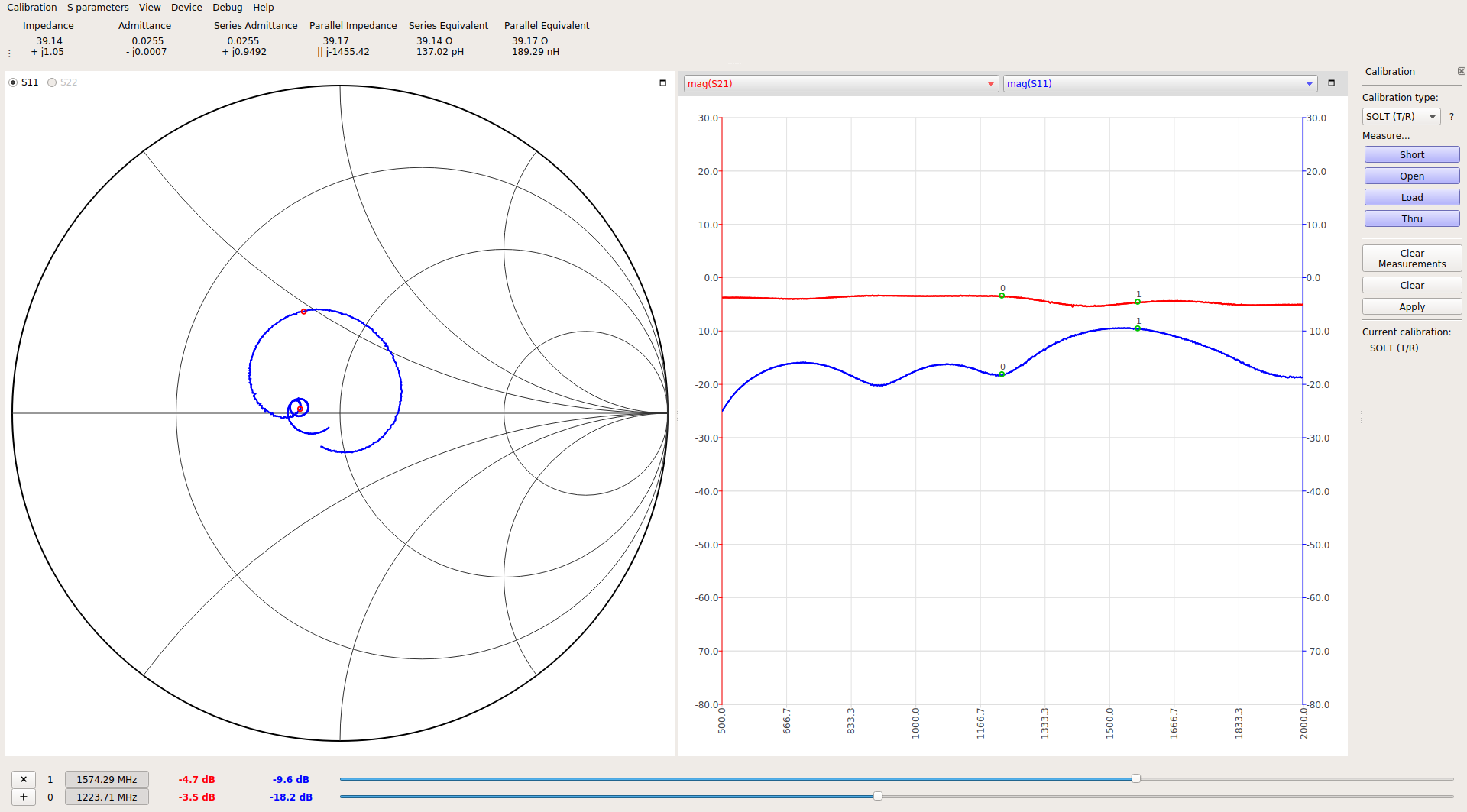
The figure below shows a measurement of the splitter in the VNA, with the third port terminated with a load. It performs quite well in the DME band, but even though I think it was marketed for GPS, it doesn’t perform so well at 1575.42 MHz (the GPS L1 frequency).
Complete hardware set up
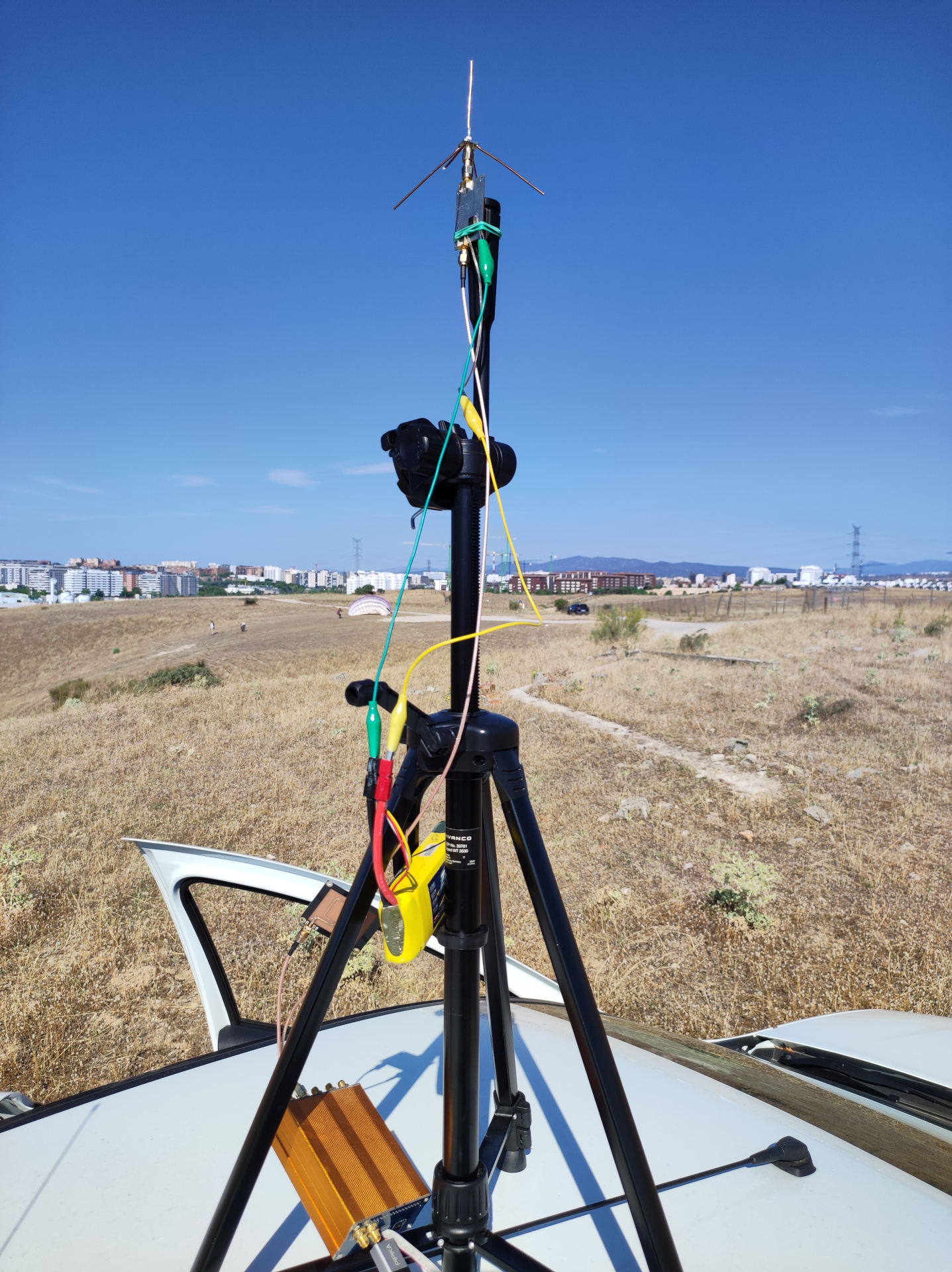
The antenna is connected through the LNA and the splitter to the two RX channels of the LimeSDR. I placed everything on a camera tripod on the roof of my car and used a LiPo battery to power the LNA. The following photo shows how everything looked during the recording.
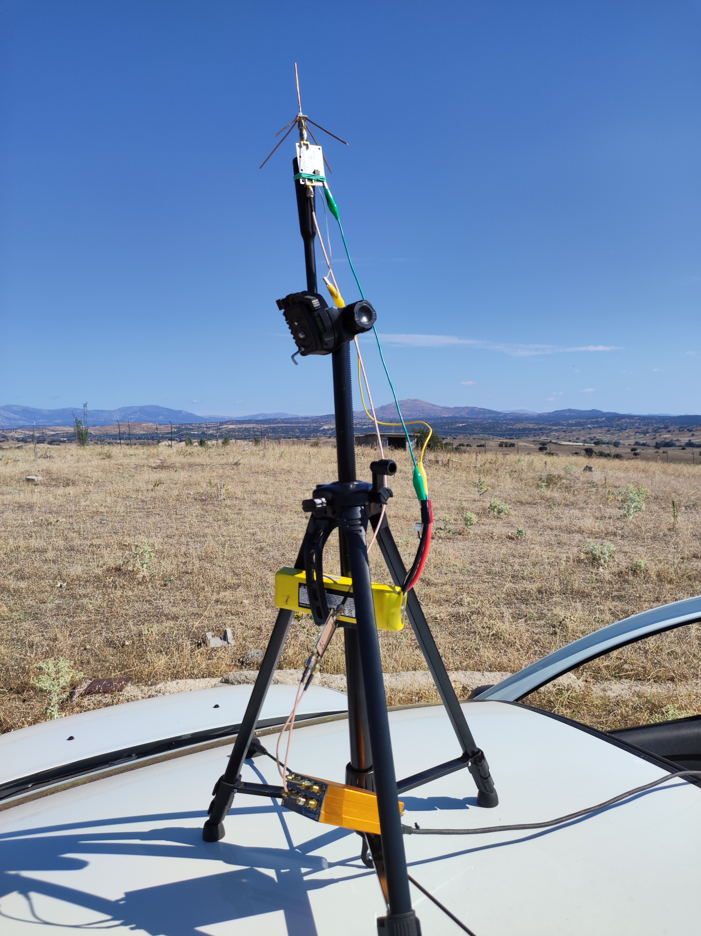
This shows the view towards the CNR VOR-DME station. The buildings are in the line of sight towards the VOR-DME, but there are no terrain obstructions behind them.
LimeSDR configuration
I have used LimeSuiteGUI to prepare the LimeSDR configuration. This configuration can then be loaded in GNU Radio using gr-limesdr. The configuration file can be found here.
I have found that it is somewhat tricky to set up from scratch a configuration in LimeSuiteGUI that uses decimation in the RXTSP. The HBD ratio in the RxTSP tab (which controls the decimation applied in the RXTSP) and the Rx clock divider in the LimeLight & PAD tab (which controls when the digital interface outputs a sample) need to be set to matching values. Otherwise samples are duplicated or missing in the output. However, it turns out that for a HBD ratio of 2^5 (which is what I’m using to reduce the 80 Msps ADC sample rate to 2.5 Msps), the Rx clock divider needs to be set to 7. The way I’ve figured this out is by configuring the LimeSDR to 2.5 Msps in GQRX (which automatically sets a decimation of 2^5) and then stopping GQRX and examining the configuration in LimeSuiteGUI. This works because GQRX doesn’t clear the configuration when it stops.
The important points to configure in LimeSuiteGUI are the following:
- In the CLKGEN tab, the CLK_H is set to 320 MHz. Together with a decimation of 4 this produces an RXTSP and TXTSP frequency of 80 MHz.
- In the SXR tab, the RX LO frequency is set to 1175 MHz, which is the midpoint of the aircarft-to-ground and ground-to-aircraft frequencies of this DME channel.
- In RxTSP tab, the HBD ratio is set to 2^5, and the NCO is set to 31.5 MHz. Channel A is set to upconvert (which shifts the frequency up), and channel B is set to downconvert (which shifts the frequency down)
- In the RBB tab, the RX filter bandwidth is tuned to 70 MHz. Experimentally it seems that this bandwidth refers to the full IQ bandwidth, so the lowpass filter cut-off is at 35 MHz.
- The gains are adjusted in the field for appropriate signal levels. I have ended up using a PGA gain of 6 dB (RBB tab), an LNA gain of Gmax-12 dB, and a TIA gain of Gmax-3 dB (RFE tab).
- RX IQ imbalance calibration is done in the field.
Note that, except for the CLKGEN and SXR setttings, all these settings need to be applied independently to each of the two channels.
In hindsight, the decision to set the LO frequency exactly at the midpoint between the air-to-ground and ground-to-air channels might have not been the best. Since this causes the two channels to be at symmetric frequencies in baseband, any IQ imbalance will cause some power from the signals from one channel to appear in the other. Offsetting the LO frequency by a few MHz would prevent this. However, this doesn’t seem to be a problem in practice. An advantage of setting the LO frequency in the midpoint is that the two channels then have a more similar response in the analog baseband, since they have the same analog baseband frequency.
GNU Radio flowgraph
A GNU Radio flowgraph is used to load the LimeSDR configuration and record data to disk.
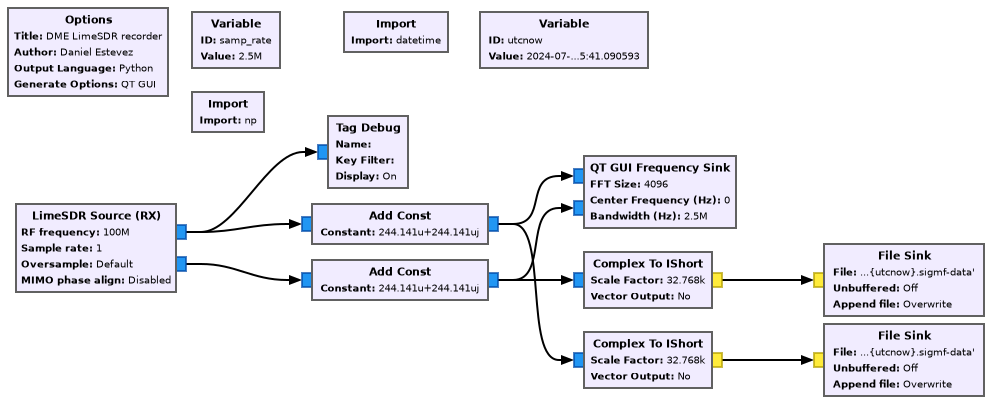
The output of the LimeSDR has a small DC spike even though we are using the NCO (so it is not the ADC DC spike). I think the reason is poor rounding in the digital signal chain. Adding 1/2**12 to each channel fixes this. This is why the Add Const blocks are present.
The Tag Debug block is used to detect lost samples, since the LimeSDR Source emits an rx_time each time that samples are lost.
The LimeSDR configuration file is loaded in the LimeSDR Source block in the Advanced tab, File option. Since we are using a configuration file, most of the other parameters in this block do not matter, as they are overwritten by the configuration file.
Since the LimeSDR doesn’t have a nice timestamp synchronization API as UHD does, timestamping of the files is done by writing the time at which the flowgraph starts running as part of the filename and also by comparing this to the modification timestamp of the file obtained using stat once the recording has stopped (this timestamp corresponds to the end of the file). This method is accurate to about 1 second, which is good enough to compare the recorded data with ADS-B data.
Recording preliminary analysis
I have performed a preliminary analysis of the recording in a Jupyter notebook to validate the recording quality. A more detailed analysis will be done in a future post.
The following figure shows the signal amplitude of the ground-to-air and air-to-ground channels in the first 100 ms of the recording. Each of the spikes we see is a pulse pair. Instead of single pulses, DME uses pulse pairs with a well determined separation between the two pulses so that the receiver can discriminate against pulsed interference.
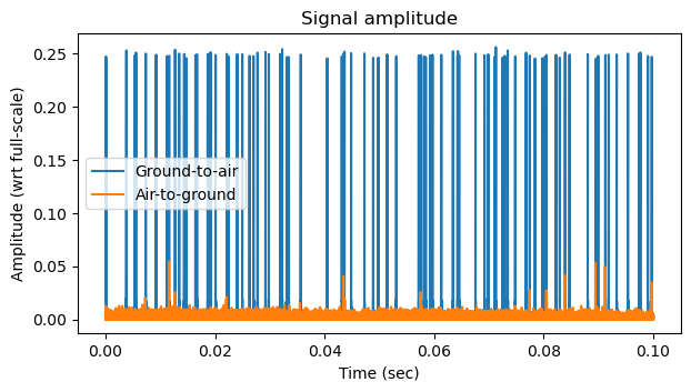
There are many more pulse pairs in the ground-to-air channel. The reason is something known as squitter. The DME transponder on ground has an AGC system that adjusts the detection threshold so that on average the transponder outputs 2700 pulse pairs per second. If there are not enough pulses received from aircraft, the transponder will trigger on random noise to generate the required amount of pulse pairs. This has several goals. It provides a constant output power to the transponder, it automatically sets the transponder threshold to a value that optimizes the sensitivity, and it degrades gracefully if the number of aircraft increases. If there are so many aircraft that the transponder receives more than 2700 pulse pairs per second, the threshold will be set high enough that the weaker aircraft are ignored. This kind of AGC system is also relatively simple to implement in hardware, so it is a very clever solution.
In this recording there are few aircraft using the DME. Each aircraft transmits around 150 pulse pairs per second when in search mode and less than 30 pulse pairs per second when in track mode, so most of the pulse pairs we see in the ground-to-air channel are squitter.
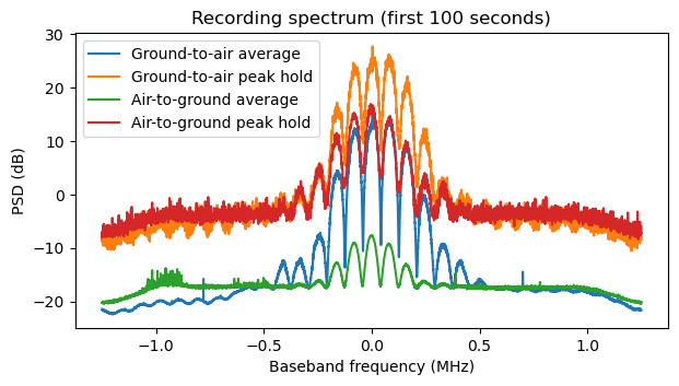
The following shows the spectrum of the first 100 seconds of the recording, using an FFT size of 4096 and a rectangular window. Both an average and a peak hold spectrum are shown for each channel. Due to the low duty cycle of the pulses (specially for the air-to-ground channel), the peak hold is often better than the average to detect the DME signal.
The following two figures show a pulse pair in the ground-to-air channel and in the air-to-ground channel. In both cases, I have plotted the pulse with largest amplitude in the first 100 seconds of the recording. The amplitude of the pulse is around 0.3 with respect to ADC full scale (or rather with respect to the full scale of the LMS7200M digital interface), so the ADC is probably still far from saturation.
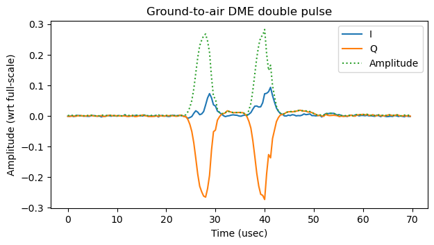
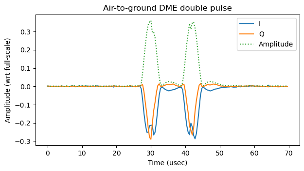
There are two DME modes: mode X and mode Y. Each mode has different parameters for the pulse pair timing. The two modes are mainly a way to support twice as many channels, since a given frequency can be used with mode X or with mode Y (although whether a given frequency is air-to-ground or ground-to-air also changes with the mode). This DME is mode X (recall that it is TACAN channel 120X), so as indicated in this webpage, the distance between the two pulses in the pair is 12 usec both for the air-to-ground and ground-to-air channels (mode Y uses different distances for air-to-ground and ground-to-air) and the transponder retransmits the pulses with a delay of 50 usec.
The shape of the pulses is somewhat ugly. The SNR is very high, so this is caused by signal distortion, not noise. In the ground-to-air channel perhaps this distortion is multipath, although in the air-to-ground pulse there seems to be an echo with a delay of ~5 usec. This corresponds to 1.5 km. I can’t think how this receiver set up could have 1.5 km of multipath for pulses coming from aircraft, so maybe the distortion is generated in the receiver hardware. Or maybe the aircraft signal is reflected in a building. Who knows.
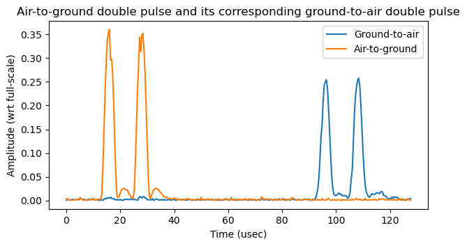
The next plot shows the same air-to-ground pulse pair, and its corresponding reply on the ground-to-air channel. The reply is received with a delay of approximately 70 usec. The transponder has a delay of 50 usec, and since my receiver is 4.58 km away from the VOR-DME station, the transponder signal takes another 15 usec to reach the receiver. Therefore, this means that the aircraft signal arrived to my receiver 5 usec before it arrived to the VOR-DME station. If we can identify which aircraft transmitted this pulse, we should be able to check that it was 1.5 km closer to my station than to the VOR-DME in this moment. This will be done in the next post.
Another interesting feature of the DME ground station is that it periodically sends an identification in Morse code. The way in which this is done is quite ingenious. To transmit a Morse dash or dot, the transponder stops listening to aircraft transmissions and replaces the squitter by a train of 1350 equally spaced pulse pairs per second. This is shown in a plot here. The transition from the squitter to the regular train of pulses is apparent.
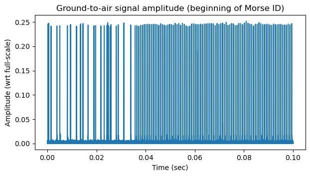
When a DME signal is received with an AM receiver such as the ones that are used for aircraft communications, even though the bandwidth of a typical AM receiver is 10 kHz and the bandwidth of the DME signal is 1 MHz, the DME signal causes a distinct sound in the AM receiver audio output. Each DME pulse pair causes a single pulse in the AM receiver audio output. This single pulse is longer, around 100 usec long, due to the reduced bandwidth of the AM receiver. The train of regularly spaced pulses sounds quite similar to a 1350 Hz rectangular wave. The value of 1350 Hz is chosen to be distinct from the tone used by VOR for its Morse ID, which is 1020 Hz.
The audio clip below shows a few seconds of DME squittter and then the Morse ID. The Morse 1350 Hz tone can be heard quite naturally. Observe that there is squitter between the Morse dots and dashes. Also note that the squitter sounds quite different from AWGN, so an AM receiver can be used to detect the presence of a DME ground-to-air signal and even to get a rough idea of its SNR, since as the signal becomes weaker, more and more AWGN will be heard in the AM receiver. This audio file was obtained with this GNU Radio flowgraph.
During the Morse identification, aircraft don’t receive valid response pulses from the DME transponder, so the DME receiver on the aircraft stops updating its distance measurement until valid transponder replies are received again.
Code and data
The GNU Radio flowgraphs and the Jupyter notebook used in this post are in this repository. The recording is published as a dataset in Zenodo.
can we decoding dme with rtl-sdr?
With an RTL-SDR you can receive a single DME channel.
This is a brilliant use of the LMS7002M’s dual RXTSP and NCO features to bypass the typical bandwidth limitations of USB3. Capturing both DME channels synchronously provides such a clear look at the transponder delay. I’ve found that when working with high-gain LNAs in these setups, managing the dynamic range is key to avoiding pulse distortion. Sometimes adding a high-quality RF Attenuator before the SDR input helps in preventing ADC clipping while maintaining the integrity of the pulse shape for TDOA analysis. Looking forward to the ADS-B correlation post!
Hi Allen, you are absolutely right that an attenuator would improve this setup by avoiding saturation. However it was difficult to foresee how the RF conditions would be when recording in the field. The TDOA analysis and comparison to ADS-B data was done already in https://destevez.net/2024/10/analysis-of-dme-signals/
Thank you so much for sharing; I gained useful information from the article.