This post is a continuation of my Artemis I series. LunaH-Map, also called Lunar Polar Hydrogen Mapper (and called HMAP by the DSN) is one of the ten cubesats that were launched with Artemis I. It is operated by Arizona State University, and its main mission was to use a scintillation neutron detector to investigate the presence of hydrogen-rich compounds such as water around the lunar south pole. Unfortunately, it was unable to perform its required lunar orbit insertion burn. Nevertheless, the spacecraft seems to be functioning well and some technology demonstrations and tests are being done with its subsystems. With some luck, there might be opportunities for this satellite to move to lunar orbit in the future.
In my observation with the Allen Telescope Array done about seven hours after the Artemis I launch I did some recordings of the LunaH-Map X-band telemetry signal when it was in communications with the DSN grounstation at Goldstone. First I did a 10 minute recording at 15:00 UTC. Then I noticed that the spacecraft had changed its modulation, so I did a second recording at 15:16 UTC, which lasted ~7 minutes. Unfortunately, I didn’t record the moment in which the telemetry change happened.
I have published these two recordings in the dataset Recordings of Artemis I LunaH-Map with the Allen Telescope Array on 2022-11-16 in Zenodo. This post is an analysis of the signals in these recordings.
Waterfalls and beamforming
The analysis of the waterfalls and signal polarization is done in the same way as for the Orion signal (see the previous post).
In the first recording, the signal modulation is PCM/PM/bi-phase-L. The carrier suppression seems quite large, as the residual carrier looks quite weak compared to the data sidebands. We can notice some weak CW tones at even multiples of the baudrate. These are most likely caused by amplitude modulation in the I component of the phase-modulated carrier, which happens when the edges of the telemetry symbols are lowpass filtered. Such filtering causes smooth and non-instantaneous crosses through zero of the modulating waveform, which in consequence makes the amplitude of the I component increase slightly at these instants.
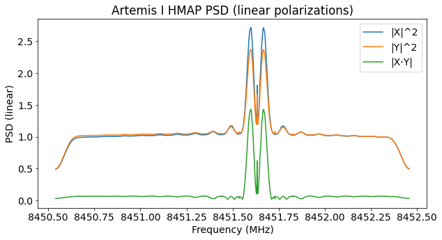
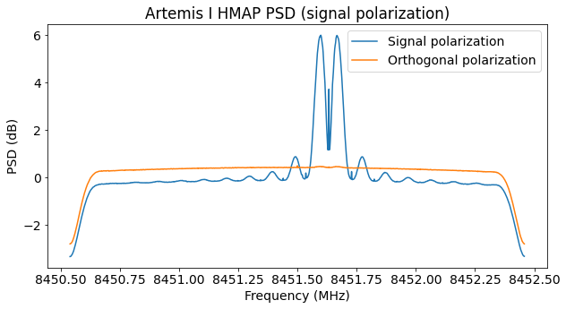
The power spectral density shown above correspond to antenna 1a (the recording was done with antennas 1a and 5c in dual linear polarization). I have adjusted the amplitude of the two polarizations so that the level of the noise floor is the same. The signal is stronger in the X polarization, which would indicate a signal which deviates somewhat from circular polarization (it might still be the case that the noise figure in the Y polarization is higher for some reason; I didn’t do a polarization calibration for these recordings). Nevertheless, as I did for Orion, I will assume that the polarization is circular and simply determine the phase offset between the X and Y channels, correct for that phase offset, and add both channels together.
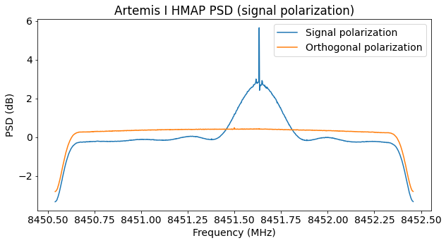
The figure below shows the power spectral densities of the signal polarization and the orthogonal polarization. Note that the noise floor is different in both polarizations. This hints at either polarized noise being present, or a high amount of polarization leakage. This is also evidenced by the fact that the noise floor of the XY cross-correlation, shown above in green, is not zero.
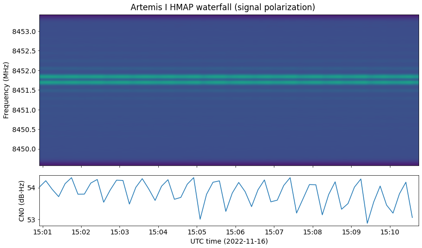
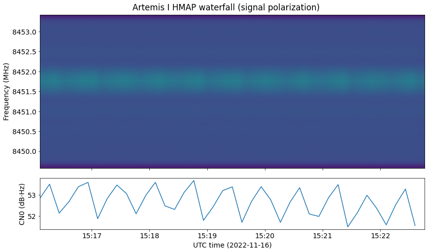
Next we have the waterfall for this recording. The CN0 is between 53 and 54 dB·Hz. It is not very apparent in this waterfall, but the signal power fluctuates because the spacecraft is tumbling.
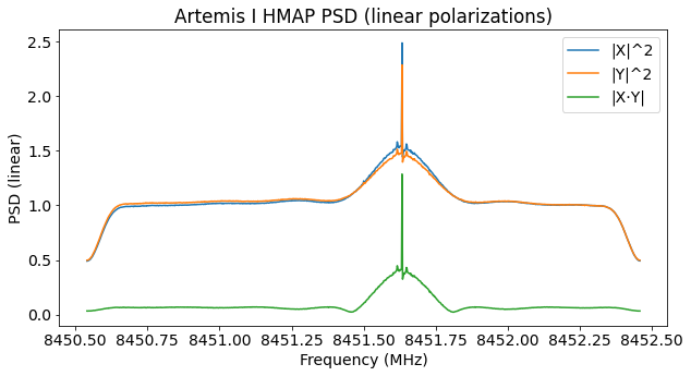
In the second recording, the modulation is PCM/PM/NRZ and uses a higher baudrate. It is possible that the change in modulation is due to the DSN routinely checking the communications system and trying different data rates at the beginning of the mission.
The figure below shows the power spectral density for antenna 1a. It is noteworthy that the modulation seems to have some artefacts. There are two small CW carriers, and the right hand side of the spectrum seems to be notched near the residual carrier. These imperfections can be seen better in the plot of the signal polarization below. I don’t know what causes them.
The next figure shows the waterfall. The CN0 is around 52 to 53 dB·Hz, and some fading is apparent. We will see that this is caused by the spacecraft being tumbling.
As we will see, in this higher data rate mode, the SNR from one antenna is not enough to decode almost all the frames. Therefore, I have beamformed the two antennas with which I recorded: 1a and 5c. I have determined the parameters used for beamforming by hand in a similar way to how I calibrate the gain and phase offset for polarization synthesis. For beamforming, first the signal polarization is synthesized separately for each antenna. Then, the gain offset between the two antennas is determined and compensated. The phase offset changes with time as the position of the spacecraft keeps changing with respect to the baseline (mainly due to the rotation of the Earth). Therefore, to correct the phase offset, I have determined a frequency (Doppler difference between the two antennas) and an initial phase. Additionally, a time difference (group delay) between the two antennas needs to be determined and corrected. For simplicity, I have used a delay of an integer number of samples to implement this correction. The way to determine the appropriate delay correction is to look at the slope of the phase difference between the two antennas versus frequency.
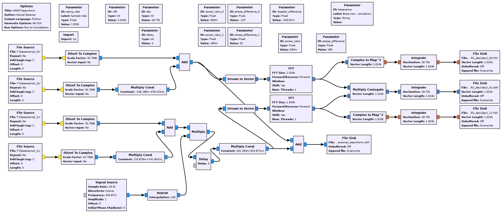
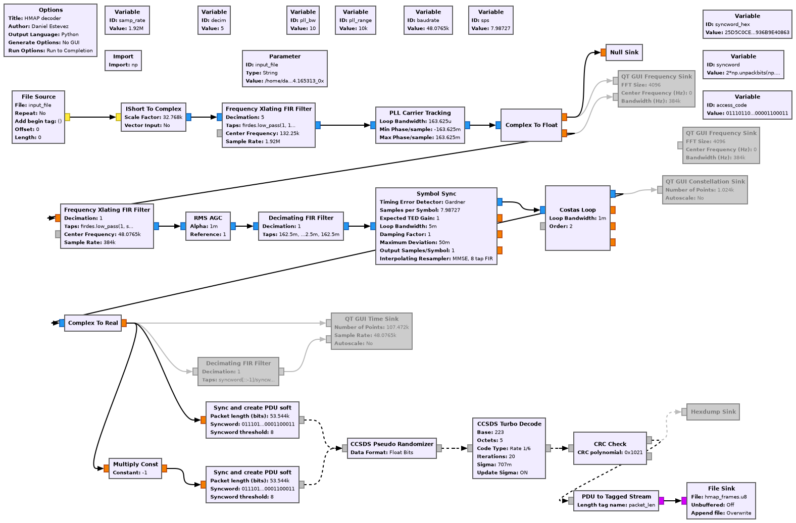
After these parameters have been determined and corrected, the two signals can simply be added. The determination of the beamforming parameters and the beamforming itself is done with the GNU Radio flowgraph shown here (hmap_beamform.grc).
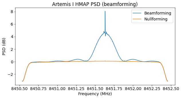
To assess the quality of the beamforming, I also formed the difference of the two signals, which corresponds to nullforming in the direction of the signal. If the beamforming is done properly, this should remove all the signal power. We can see the power spectral density for the beamforming combination and the nullforming combination below.
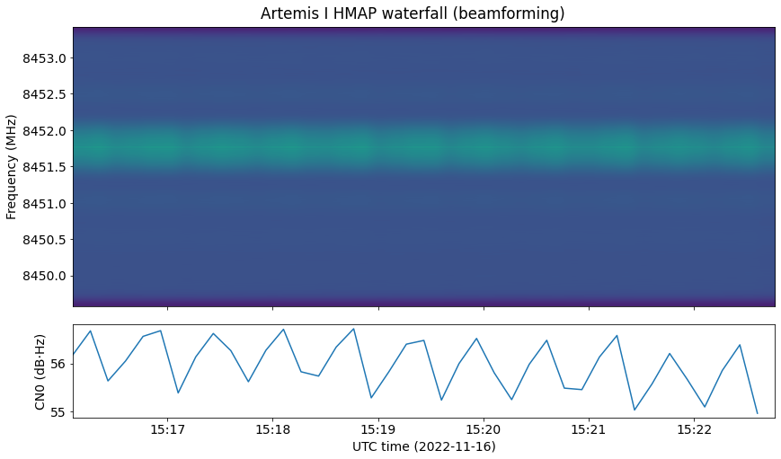
The next figure shows the waterfall for the beamformed signal. The CN0 is now between 55 to 56 dB·Hz, so we have gained 3 dB of SNR. This is to be expected for the beamforming combination of two antennas with the same characteristics.
Modulation and coding
In the first recording, the modulation is PCM/PM/bi-phase-L with a symbol rate of approximately 48.0765 kbaud. This means that the telemetry data is Manchester encoded and phase modulated with residual carrier. This gives rise to two data sidebands adjacent to the carrier. In the second recording the modulation is PCM/PM/NRZ with a symbol rate of approximately 255.1 kbaud. This means that the telemetry is directly phase modulated on the carrier, so there are no sidebands (but there is still a residual carrier).
The baudrates given here look a bit strange, as they are not round numbers. The measurement I have done of these symbol rates is not very precise, and is affected by Doppler. In any case, there is nothing wrong with them. The change from using bi-phase-L to using NRZ is pretty common in order to save occupied bandwidth when going to a higher symbol rate (on the other hand, lower symbol rates should avoid using NRZ to prevent causing too much interference to the PLL that locks to the residual carrier).
The coding is CCSDS Turbo Code with 1115 information bytes in both cases. In the bi-phase-L case, the rate is 1/6, and in the NRZ case the rate is 1/2. Therefore, the bi-phase-L mode gives a data rate of about 8 kbps, while the NRZ mode gives about 127.5 kbps. This represents a 16x increase in data rate.
From a perspective of Eb/N0 performance, r=1/6 Turbo Code with 1115 byte information codewords is the best FEC algorithm defined by CCSDS. Therefore, this configuration is very commonly used by current deep space missions unless there are additional constraints to take into account (such as having too long codewords at very low data rates or having too much occupied bandwidth at high symbol rates). In the case of the the NRZ mode, the change to r=1/2 degrades the Eb/N0 performance slightly, but reduces the occupied bandwidth by 3. It seems that the modulations of this spacecraft are designed to fit into around 0.5 MHz to 1 MHz.
The flowgraphs used for decoding the two modes are shown below (hmap.grc and hmap_nrz.grc). Both are quite similar. The only differences between them are in the demodulator, due to the changes required between bi-phase-L and NRZ, and in the size of the Turbo codewords and the ASM.

Something interesting is that in the NRZ mode we need to invert the symbol stream. This is because LunaH-Map transmits the bit value 0 as an advance in the phase of the signal.
In the bi-phase-L mode, the SNR in a linear polarization of one antenna is good enough to give error-free decoding, so I haven’t worried to synthesize the correct signal polarization. In the NRZ mode, due to the much higher data rate we need to use the correct signal polarization and beamform two antennas to obtain almost error-free decoding.
The Turbo decoder, which uses the block from gr-dslwp, is pretty slow. In the NRZ mode it takes a while to process the whole recording (it is a few times slower than real time).
AOS frames
The decoded frames are analyzed in two Jupyter notebooks: one for the bi-phase-L mode, and another for the NRZ mode.
In both the bi-phase-L mode and the NRZ mode, the frames are CCSDS AOS Space Data Link frames. They have an FECF (frame error control field; CRC-16), which is checked and stripped by the GNU Radio flowgraph. There is no Operational Control Field or Transfer Frame Insert Zone. The frames use Spacecraft ID 0xd6, which as expected is assigned to LunaH-Map in the SANA registry. Interestingly, this spacecraft ID assignment is only for the return (space to ground) link. The forward (ground to space, telecommand) link has assigned 0x34a. More often than not, spacecraft use the same ID for the forward and return links.
There are two virtual channels in use, virtual channel 2, which carries telemetry data, and virtual channel 63, which carries only idle data (this virtual channel is always reserved for idle data).
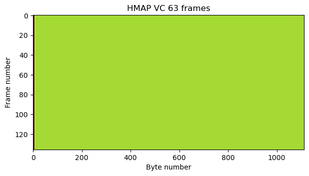
The frames in virtual channel 63 carry an M_PDU header with a first header pointer value of 2046, which indicates that the packet zone carries only idle data. The packet zone is filled with the byte 0xdc, which seems to be the padding byte used by this satellite. The figure below shows the raster map of all the virtual channel 63 frames decoded from the first recording.
The frames in virtual channel 2 use M_PDU to carry CCSDS Space Packets. In the first recording, there are only two APIDs being used by these space packets: APID 66 and APID 2047. APID 66 carries telemetry data (presumably real-time telemetry), and APID 2047 carries idle packets (this virtual channel is reserved for idle packets).
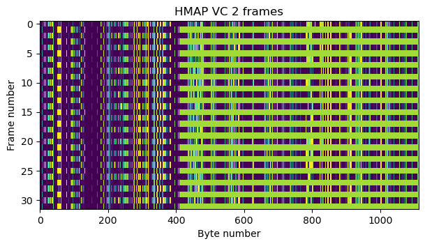
The sequence in which these packets are transmitted is always the same. First, a 1501 byte packet from APID 66 is sent. This packet occupies one full AOS frame and a part of the next one. The remaining part of the second AOS frame is occupied by a 709 byte idle packet using APID 2047. This behaviour can be seen in the next figure. It shows the first 32 frames from virtual channel 2 decoded from the first recording. The payload of the idle packets is filled with 0xdc bytes, which appear in green in the raster map.
Interestingly, all the Space Packets sent by LunaH-Map have the packet sequence count field set to zero. This means that all the idle packets are exactly identical. The packets in APID 66 have the secondary header flag set to true, but I haven’t looked very carefully to try to understand the format of the secondary header. It seems that there is a counter, which is probably a time code. The packets in APID 2047 have the secondary header flag set to false as expected.
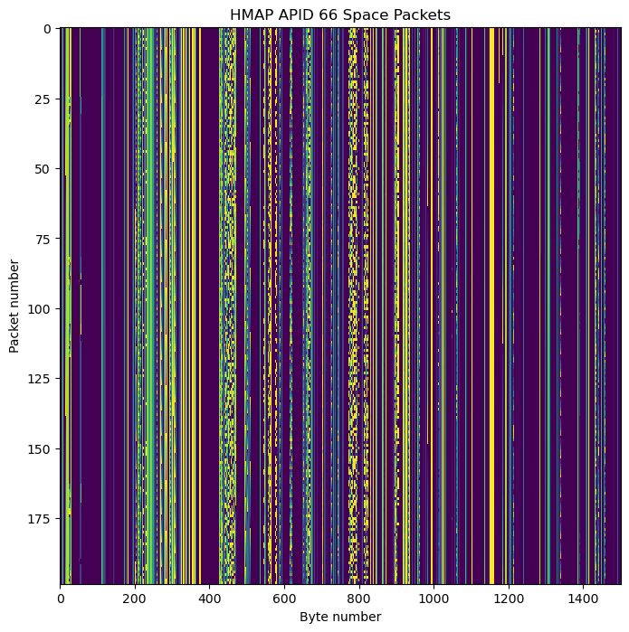
The figure below shows the raster map for the packets in APID 66. We will look at some of their contents later.
The second recording is more interesting, because there is an operational change halfway through the recording. With this recording I have taken care to keep track of the timestamps of each frame and space packet. This is done manually by using the timestamp of the IQ data, taking into account the nominal duration of a frame at 255.1 kbaud rate, and assigning to each space packet the timestamp of one of the frames that carries it. This will not give perfect results, but is good enough for our purposes.
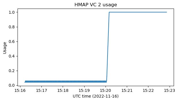
The figure below shows the usage of virtual channel 2, compared to the total bandwidth of the link. The remaining bandwidth is used by virtual channel 63. We see that at 15:20 UTC the usage changes, and virtual channel 2 passes from being using a rather low rate to occupying the link fully.
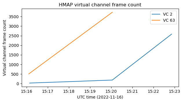
An alternative way to show this change is by plotting the virtual channel frame count of the frames we see. We note that at some point the frames from virtual channel 63 stop completely and consequently the frame count for virtual channel 2 starts increasing much faster. It is quite interesting that the frame counts at the beginning of the recording are quite small. Perhaps they were reset when the spacecraft changed its modulation. The first virtual channel frame counts that we see are 26 and 504 for virtual channels 2 and 63 respectively. This amounts to a total of 530 frames, which take approximately 37 seconds to transmit.
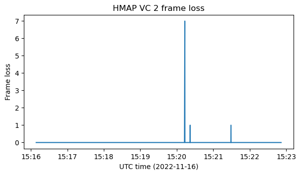
In the first recording the decoding was completely error-free. However, in the second recording even though I have taken care to beamform two antennas and optimize the decoder parameters, we have lost 9 frames out of a total of 5777. All the lost frames belong to virtual channel 2, as shown in the figure below.
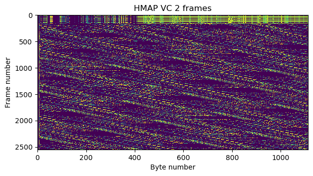
If we plot the raster map of the frames in virtual channel 2 in the second recording, we see that the pattern begins as in the first recording, with one packet from APID 66 followed by an idle packet, but then there is something different. This corresponds to the appearance of packets from APID 1080 as the operational change happens and virtual channel 2 begins to use the full link capacity.
The change is illustrated better by the following plot, which shows the usage of each APID within virtual channel 2. At first, there is a 50% usage for both APID 66 and APID 2047, basically because a frame from each APID is sent alternatively. When the happen changes, APID 2047 completely disappears, and APID 1090 appears and starts using most of the bandwidth. It is interesting that there is a transient where it appears that too many packets from APID 1090 are being sent, restricting the rate of APID 66. This is perhaps due to some queuing in the transmitter.
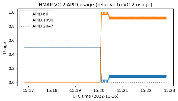
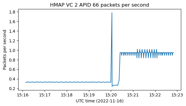
This figure doesn’t tell the whole story, because it doesn’t take into account the change in the occupancy of the virtual channel with respect to the total link bandwidth. It is instructive to plot the number of packets per second sent in APID 66, which is simply calculated by measuring the time different between consecutive packets in this APID. We see that even though in the plot above it seems that the rate of APID 66 decreases, it is actually increasing from around 0.35 packets per second to nearly 1 packet per second.
With all this data, we now have a better idea of what the operational change at 15:20 UTC implies. It seems that first only the modulation and coding was changed to allow a much faster data rate, but the configuration for what telemetry is being sent wasn’t changed, so only a small fraction of the total link bandwidth was being used. After checking for a few minutes that things seemed to work correctly, a new configuration was enabled that transmits APID 66 telemetry somewhat faster and spends the remaining link capacity to send APID 1090, which as we will see below, seems to be real time high-rate telemetry. What doesn’t completely check up is that with the bi-phase-L mode the rate at which APID 66 was sent was at about 0.66 packets per second, while in the first part of the second recording a lower rate of about 0.35 packets per second is used.
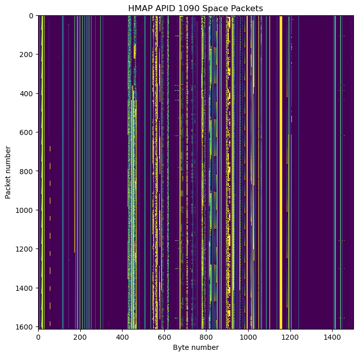
These packets in APID 1090 have the same length as those in APID 66: 1501 bytes. They also have the secondary header flag enabled and the packet sequence count set to zero. The next figure shows the raster map for the packets in this APID. We see that all the packets have the same structure, which looks vaguely similar to that of APID 66, but is really different.
ADCS telemetry
I have been taking a look at raster maps of APID 66 and APID 1090 to try to find telemetry channels that looked interesting. I’ve been lucky enough to find what I think is some telemetry from the ADCS (attitude determination and control system), including some quaternions. I haven’t fully understood all of this data, but at least I’m quite confident on how I’m interpreting some of it.
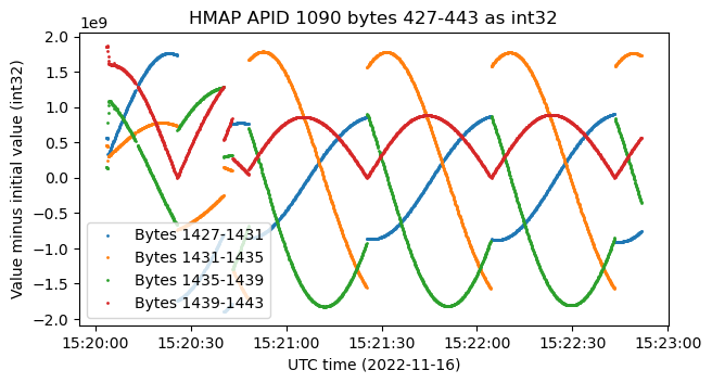
Let’s start by looking at some int32 big-endian fields in APID 66. Here I’m using the data from the second recording, but the data from the first recording is very similar. There are four int32 fields that are separated by four fields filled with zeros. These increase/decrease at a linear rate more or less. In the figure, I have plotted each field minus its initial value, because the fields have very different offsets.
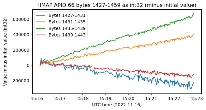
What is special about these four fields is that if we calculate their sum of squares, we obtain a constant. Any time that this happens with four numbers in spacecraft telemetry, we can start to suspect that we’re looking at quaternions. The analysis I will do in what follows is quite similar to what I did some years ago with the ADCS telemetry for Tianwen-1. However, the analysis here will be more difficult and not as complete because we don’t have such a simple situation as in the case of Tianwen-1, which was executing a certain rotation about the spacecraft body’s Y axis.
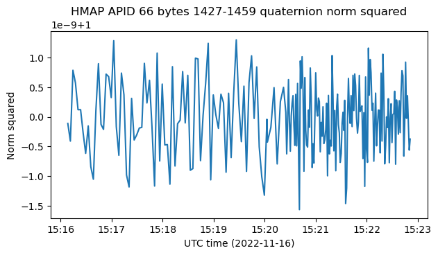
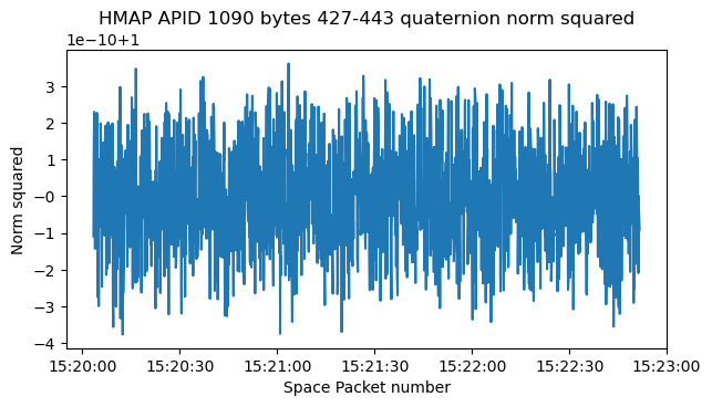
The scale factor for these quaternions is \(10^9\). I am yet again intrigued by why people don’t use scale factors which are a power of two for quaternions. Tianwen-1 used int16 quaternions with a scale factor of \(10^4\). The figure below shows the quaternion norm squared once we have applied the correct scale factor. We see that the norm only deviates from 1 by around \(10^{-9}\). This small deviation is to be expected because of quantization errors in the int32 values.
Now we have some ambiguity about the coordinate order for these quaternions. The most straightforward order would be \(1\), \(i\), \(j\), \(k\), but “scalar last” format (\(i\), \(j\), \(k\), 1) is also a popular format. I am not sure about what is the correct ordering here. There are some hints that support scalar first format, and others that support scalar last (we will get to these when we look at APID 1090). In the appendix near the end of the post I have included some details about what happens if we permute the coordinates of a quaternion, which is relevant here in case we mess up the ordering of the coordinates. To do the plots below, I will assume that the data is transmitted in scalar first coordinates.
If we denote these quaternions by \(q(t)\), where the variable \(t\) represent time, we can compute the relative rotation between the initial time \(t = 0\) and the other times by calculating \(q(t)q(0)^{-1}\). This will also be a quaternion that represents a rotation. We can get the rotation axis by taking its imaginary components and normalizing them. The coordinates of the resulting vector are shown below.
We see that the rotation axis pretty much stays constant over time (except near the beginning, where the problem of finding the axis is ill-conditioned because \(q(t)q(0)^{-1}\) is close to the identity). Seeing that we get a constant axis of rotation is a good consistency check for our understanding, because most rotations that would be represented as quaternions change by rotation along a constant axis when studied over short enough time intervals.
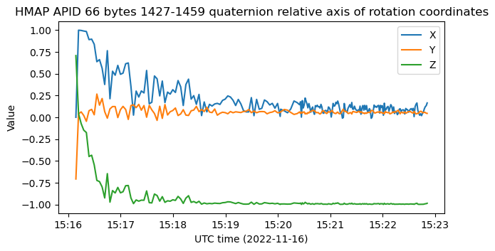
The axis of rotation is also pretty close to the -Z axis. This is also a good clue, because it is quite unlikely that we get a rotation axis that is aligned to one of the coordinate axes just by chance. This clue supports the scalar first order for the quaternion coordinates. If we interpret them in scalar last order, then we get a completely different axis that is not aligned with the coordinate axes.
We can also compute the rotation angle of this rotation. The surprising thing is that the rotation angle is very small. This was to be expected, because the change of the quaternions themselves is also very small. That is the reason why I plotted them subtracting their initial value. If I plot them without this subtraction, they just look like constant values. Still, the rotation angle looks good because it gives a constant angular speed of rotation. Most rotations should look like this.
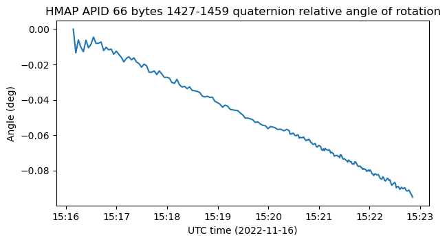
The rotation rate is -0.00023 deg/s. At this rate, it takes 17.6 days to complete a revolution.
So what do these quaternions encode? I’m pretty sure it’s not the spacecraft attitude. As evidenced by the signal fading, and also by some quaternions in APID 1090 that we will study next, the spacecraft is tumbling. I don’t have a good explanation, but at least I have some intuitions.
The fact that the rotation period of 17.6 days is on the order of the period of Earth orbits in the lunar region (compare with the orbital period of the Moon, which is ~27 days) might be a hint. This might be some kind of target attitude or an orientation of some sorts that involves some celestial bodies (perhaps the Moon) in its definition. Therefore, the attitude changes slowly as the satellite and these celestial bodies travel around its orbit. The fact that the rotation axis is very close to the -Z axis also supports this idea. All these objects would be moving close to the XY plane, so the changes in the relative positions of these objects look like a rotation about the Z axis.
To give an example of the kind of attitude descriptions I have in mind, let’s think about the attitude defined by one of the spacecraft axes pointing towards the sun (to aim its solar panels), another towards the Earth (to aim its antenna), and the third axis completing a right-handed system. This attitude would slowly rotate as the spacecraft travels on its transfer orbit to the Moon. I’m not implying that this attitude is what is encoded by these quaternions, but I wouldn’t be surprised if it’s something fitting a similar description. Still, this brings up the question: if the quaternions are described by some mathematical model rather than from some measurements, why do they look so noisy?
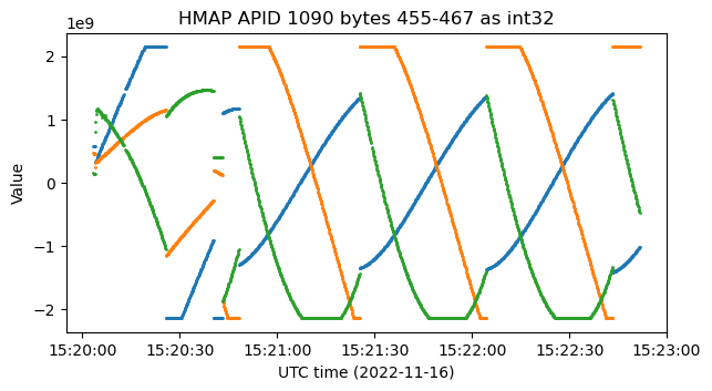
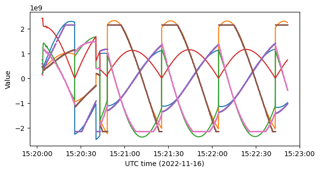
Now let’s look at some quaternion data from APID 1090. Here are four adjacent int32 big-endian fields that show some sinusoid-like behaviour.
If we scale them by dividing by \(2\cdot 10^9\), and compute the sum of modulus squared, we get a constant value of one (plus some quantization noise).
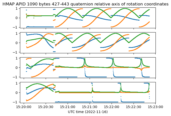
The correctly scaled values are shown below, labeled as quaternion coordinates using the scalar first order.
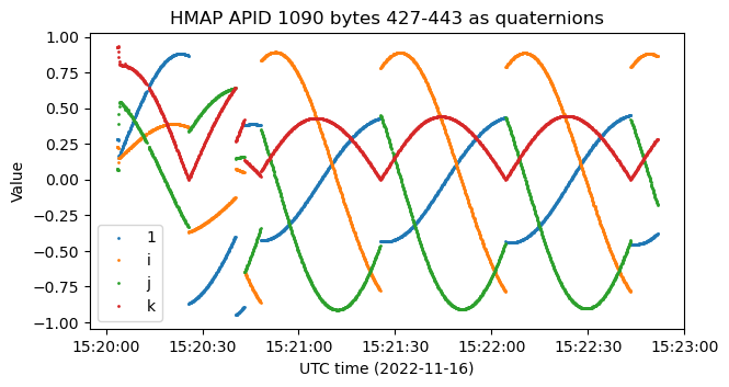
Something we note is that there are some jumps in the values. Several of these jumps are caused by a sign convention. Note that the quaternions \(q\) and \(-q\) represent the same rotation. Therefore, we can change sign at will in our quaternion representations. We might want to change the sign as appropriate to keep the sign of one of the coordinates positive. This is what happens here with the last field (plotted in red). Note that it is always positive, and that when it reaches zero, the remaining fields change sign.
Here I have labeled the red field as \(k\), following the scalar first ordering. However, the fact that this field is always positive supports the scalar last ordering. A quaternion representing a rotation can be written as\[\cos\frac{\theta}{2} + (v_x i + v_y j + v_z k)\sin\frac{\theta}{2},\]where \((v_x, v_y, v_z)\) is a unit vector that represents the axis of rotation and \(\theta\) is the angle of rotation. If we restrict ourselves to rotations with \(-\pi \leq \theta \leq \pi\), then the real part is always positive. When the rotation the rotation angle goes, say, past \(\pi\), we represent a rotation of angle \(\pi + \varepsilon\) as a rotation of angle \(-(\pi – \varepsilon)\) with the same axis. This amounts to keeping the scalar component positive and flipping the sign of the imaginary components.
Still, the quaternions in APID 66 provided some support for the scalar first order. It might be that the quaternions in APID 1090 use a different order, in the same way that they use a different scale factor. Nevertheless, I will follow also the scalar first order for APID 1090. This doesn’t affect the main conclusions, as shown in the appendix at the end of the post.
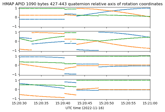
There are some other jumps in the quaternions around 15:20:45 UTC that do not correspond to jumps caused by keeping the red component positive. As we will see now, these correspond to jumps in the axis of rotation. There are actually four distinct regions that have four different axis of rotation. To study these regions, we select time instants \(t_1\), \(t_2\), \(t_3\), \(t_4\) in each of the four regions and compute the quaternions \(h_j(t) = q(t)q(t_j)^{-1}\). Then we extract and plot the axis of rotation for each of these. These are plotted in the figure below.
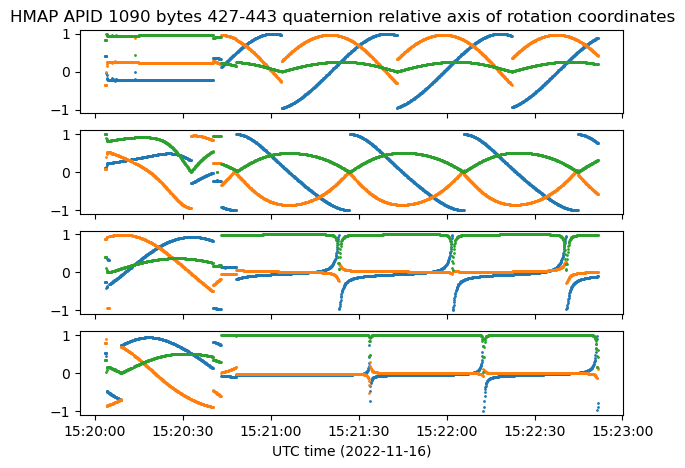
We see that in fact the axis of rotation stays constant within the region in which the point \(t_j\) was picked, but changes in all the other regions. The plot below provides a better look at what happens around 15:20:45 UTC. Note that the axes in regions 3 and 4 are close.
The next figure shows the angle of rotation of each of the quaternions \(h_j(t)\). They are coloured in blue for \(j = 1\), orange for \(j = 2\), green for \(j = 3\), and red for \(j = 4\). Within the region in which each of the quaternions \(h_j(t)\) applies, the rotation angle changes at a constant rate. The rate is very similar for all of the regions. Therefore, the conclusion is that the four regions describe rotations with different axis but the same rate. The rotation rate is 1.56 revolutions per minute.
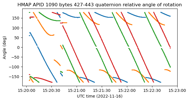
This rotation rate corresponds to the tumbling rate of the spacecraft. In fact, we can compare the plot above with the waterfall of the signal, reproduced here again for convenience. Between 15:20 and 15:23 the quaternions perform ~4.5 rotations. Looking at the fading pattern in this interval, we also see ~4.5 periods of the pattern.
Therefore, it seems that APID 1090 is high-rate real-time telemetry. Since most of the link bandwidth is dedicated to this APID, we see that this high-rate telemetry is sent at a rate of ~10.48 Hz, since the net data rate taking into account the AOS headers and FECF is ~15737 bytes/s, so a 1501 byte Space Packet takes 0.095 seconds to be sent.
I am left wondering about the four zones in the quaternion data and the sudden changes in the rotation axis. These are clearly non-physical. The spacecraft attitude cannot jump instantly, and looking at the signal the fading pattern looks the same all along. One possible idea is that the ADCS is having troubles trying to figure out the rotation axis in an inertial frame. Using gyroscopes, it is easy to find the rotation rate and the axis in the spacecraft body frame. But the representation of the axis in an intertial frame, or in other words, the spacecraft absolute orientation, is more difficult to determine (specially if the spacecraft is spinning, in which case perhaps the star tracker cannot work correctly). Maybe the ADCS is struggling to find this and its solution jumps, but it is always consistent with the gyroscope data (which would set the rotation rate). Another possible idea is that the data is being output using different reference frames, though I can’t think of a reason why the system would work in this way.
There is still some more guesswork that can be done with this quaternion data, but this starts to rely more on us choosing the correct permutation for the coordinates (scalar first versus scalar last). Typically, the spacecraft attitude quaternions \(q(t)\) would represent the rotation from the spacecraft body frame to some inertial frame, such as ICRF. Therefore, the quaternions \(h(t) = q(t)q(t_0)^{-1}\) represent a relative rotation in inertial coordinates. It can be understood in the following way. We take a vector in inertial coordinates, attach it rigidly to the spacecraft at time \(t_0\), let time run until \(t\), and then look at the inertial coordinates of the vector. The axis of this rotation is hence the rotation axis in inertial coordinates.
However, if instead we look at the quaternions \(r(t) = q(t)^{-1}q(t_0)\), these represent a relative rotation in spacecraft body coordinates. Their interpretation is as follows. We take a point in the spacecraft, detach it from the spacecraft at time \(t_0\) so that the point stays fixed in inertial space, let time run until \(t\), and then reattach the point the the spacecraft. The spacecraft has rotated and the point has stayed fixed, so the point is now reattached to a different position in the spacecraft. The quaternion \(r(t)\) represents the movement of this point. It is a rotation in spacecraft body coordinates, and its axis is the spacecraft rotation axis in body coordinates.
It turns out that if we take the scalar last ordering for the APID 1090 quaternions and compute the axis of rotation in spacecraft body coordinates using this technique, then the axes we get in each of the four regions look quite similar. Moreover, they are close to the -X axis. The figure below shows the coordinates of these axes of rotation.
These ideas might support that the scalar last ordering is the correct one for these quaternions, but I’m not sure how much of all of these could just be a coincidence.
There are other telemetry channels in APID 1090 that seem to be related to the ADCS quaternions that describe the spacecraft attitude. The next figure shows three int32 channels that come after the quaternion data. They seem to clip at some particular amplitude, and follow curves very similar to those of the quaternions.
The following figure shows a comparison where the quaternions multiplied by a factor of 1.3 (which has been found testing by hand) and these three channels are plotted in the same plot. We see that the three channels more or less follow the three first coordinates of the quaternions (but not quite exactly), except when they clip. I have no idea of what these three channels represent. The only remark that comes to mind is that the last quaternion coordinate (which is the one not followed by any of these three channels) is somewhat redundant if we follow the convention that it must always be non-negative, because its value can be derived from the other coordinates and the fact that the quaternions have unit norm.
We also have 6 telemetry channels most of which describe sinusoids. These sinusoids have the same frequency that the rotation of the ADCS quaternions. It seems that there are redundant channels, as channels 0 and 4, 1 and 5, and 2 and 6 have almost the same data.
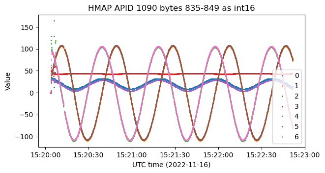
The next figure plots some pairs of these channels as we would see them on an X-Y plot on an oscilloscope. This shows that channels 5 and 6 are in quadrature and have the same amplitude, and that channels 4 and 6 are in phase, but have different amplitudes (and channel 4 has a non-zero offset).
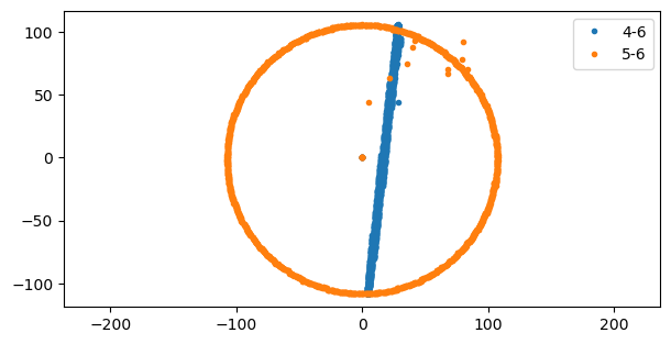
I don’t know exactly what are these sinusoids measuring. It is clear that they are related to the spacecraft rotation, but there are many ways in which one can obtain sinusoids from a rotation (anything that involves projections on a vector). I don’t have a conclusive idea to interpret them.
Appendix: permutations of quaternion coordinates
In this appendix we treat how a quaternion that describes a rotation in \(\mathbb{R}^3\) is affected by a permutation of its coordinates. We will cover a slightly more general setting. Given a quaternion\[q = x_0 + i x_1 + j x_2 + k x_3,\]we consider the quaternion\[r = \varepsilon_0 x_{\sigma(0)} + i \varepsilon_1 x_{\sigma(1)} + j \varepsilon_2 x_{\sigma(2)} + k \varepsilon_3 x_{\sigma(3)},\]where \(\varepsilon_n \in \{-1, 1\}\) and \(\sigma\) is a permutation in \(\{0, 1, 2, 3\}\).
If \(\sigma(0) = 0\), then the quaternion \(r\) describes the same rotation as \(q\), but possibly in a different frame of reference. In fact, since \(r\) and \(-r\) describe the same rotation, we may assume that \(\varepsilon_0 = 1\). Then the action of \(\sigma\) and the signs \(\varepsilon_n\) for \(n = 1, \ldots, 3\) amount to a permutation and possibly a change of sign of the coordinate axes. We see that there is an orthogonal transformation that maps one coordinate frame into the other. When passing from \(q\) to \(r\), the axis of rotation is mapped by this transformation, and the angle of rotation stays the same.
In order to study the case \(\sigma(0)\neq 0\) it is enough to consider the case when \(r = qi = -x_1 + i x_0 + j x_3 – k x_2\), since any other case can be obtained by a composition of this transformation and transformations were \(\sigma(0) = 0\). In this case, it is apparent that \(r\) describes a different rotation. For instance, in the case when \(q = 1\), which describes the identity transformation, we have \(r = i\), which corresponds to a rotation of angle \(\pi\) about the X axis. This rotation can be understood as the map that fixes X and sends Y to -Y and Z to -Z. The general case is simply a composition of this rotation followed by the rotation described by \(q\).
If we consider the relative change between two quaternions \(q_1\) and \(q_2\), which is given by \(q_2 q_1^{-1}\), and transform them to obtain \(r_1 = q_1 i\) and \(r_2 = q_2 i\), we see that the relative change between these two new quaternions is \(r_1 r_2^{-1}\) = \(q_1 i (q_2 i)^{-1}\) = \(q_1 q_2^{-1}\). Therefore, the relative change between \(r_1\) and \(r_2\) is the same as the relative change between \(q_1\) and \(q_2\).
In the general case when \(r_1\) and \(r_2\) are obtained by the same permutation and change of signs of the coordinates of \(q_1\) and \(q_2\), we see that the relative changes \(r_1 r_2^{-1}\) and \(q_1 q_2^{-1}\) are not equal in general, but they are always rotations with the same angle (in other words, \(|\operatorname{Re}(r_1 r_2^{-1})| = |\operatorname{Re}(q_1 q_2^{-1})|\)). This property also follows directly from a straightforward calculation. If\[q_1 = x_0 + i x_1 + j x_2 + k x_3\]and\[q_2 = y_0 + i y_1 + j y_2 + k y_3,\]so that\[r_1 = \varepsilon_0 x_{\sigma(0)} + i \varepsilon_1 x_{\sigma(1)} + j \varepsilon_2 x_{\sigma(2)} + k \varepsilon_3 x_{\sigma(3)},\]and similarly\[r_2 = \varepsilon_0 y_{\sigma(0)} + i \varepsilon_1 y_{\sigma(1)} + j \varepsilon_2 y_{\sigma(2)} + k \varepsilon_3 y_{\sigma(3)},\]then\[\begin{split}\operatorname{Re}(r_1 r_2^{-1}) &= \operatorname{Re}[(\varepsilon_0 x_{\sigma(0)} + i \varepsilon_1 x_{\sigma(1)} + j \varepsilon_2 x_{\sigma(2)} + k \varepsilon_3 x_{\sigma(3)})\\&\cdot(\varepsilon_0 y_{\sigma(0)} – i \varepsilon_1 y_{\sigma(1)} – j \varepsilon_2 y_{\sigma(2)} – k \varepsilon_3 y_{\sigma(3)})] \\ &= x_{\sigma(0)}y_{\sigma(0)} + x_{\sigma(1)}y_{\sigma(1)} + x_{\sigma(2)}y_{\sigma(2)} + x_{\sigma(3)}y_{\sigma(3)} \\&= \operatorname{Re}(q_1 q_2^{-1}).\end{split}\]
Code and data
The IQ recordings are contained in the Zenodo dataset linked at the beginning of the post. The Jupyter notebooks and flowgraphs for waterfall analysis and beamforming are in this repository. The GNU Radio decoder flowgraphs, the data files of decoded frames and the Jupyter notebooks analyzing the frames are in this repository.
You are the best Daniel!!!
Very detailed information. Always interesting as usual.
Seems, it use this radio:
Iris radio V2
https://www.nasa.gov/sites/default/files/atoms/files/brochure_irisv2_201507.pdf
https://www.eoportal.org/satellite-missions/iris-radio#iris-architecture