This post is a continuation of my series about LTE, where I decode a recording of the downlink signal of an eNB using Jupyter notebooks written from scratch. Here I will decode the PDSCH (physical downlink shared channel), which contains the data transmitted by the eNB to the UEs, including PDUs from the MAC layer, and some broadcast information, such as the SIB (system information block) and paging. At first I planned this post to be about decoding the SIB1. This is the first block of system information, and it is the next thing that a UE must decode after decoding the MIB (located in the PBCH) to find the configuration of the cell. The SIB1 is always transmitted periodically, and its contents and format are relatively well known a priori (as opposed to a user data transmission, which could happen at any time and contain almost anything), so it is a good example to try to decode PDSCH transmissions.
After writing and testing all the code to decode the SIB1, it was too tempting to decode everything else. Even though at first I wrote my code thinking only about the SIB1, with a few modifications I could decode all the PSDCH transmissions (except those using two-codeword spatial multiplexing, since my recording was done with a single antenna). I will still use the SIB1 as an example to show how to decode the PDSCH step by step, but I will also show the rest of the data.
The post is rather long, but we will get from IQ samples to looking at packets in Wireshark using only Python, so I think it’s worth its length.
SIB1
The SIB1 is transmitted with an 80 ms periodicity. There is a SIB1 transmission on subframe 5 of each radio frame with an SFN divisible by 8. Additionally, there are 3 retransmissions of each SIB1 transmission using different redundancy versions. We will talk about redundancy versions in more detail below. For the time being, it is enough to say that each redundancy version transmits a different set of bits produced by the Turbo encoder, and that a receiver can combine different redundancy versions of the same data to improve its chances of decoding. These 3 retransmissions happen on subframe 5 of each radio frame with SFN divisible by 2 but not by 8. Therefore, there is a SIB1 transmission on the PDSCH (either an original transmission or a retransmission) every 20 ms (2 radio frames).
The original transmission and its 3 retransmissions follow a fixed schedule for the redundancy version index (this is a number between 0 and 3 that is used to indicate which set of bits is taken from the Turbo encoder output). The schedule is 0, 2, 3, 1. The redundancy version index is also indicated in the PDCCH DCI corresponding to the SIB1 PDSCH transmission (see my post about the PDCCH), so we can use this as a cross-check.
As we will see below, to test that the implementation of the rate matching algorithm is correct, it is quite useful to have two transmissions of the same SIB1 (with different redundancy versions). The SIB1 transmissions can be identified in the PDCCH by their SI-RNTI (0xffff). Other SIB transmissions also use the SI-RNTI, but the SIB1 is the one that is transmitted most frequently (and with a transmission every 20 ms). Looking at the DCIs decoded in the PDCCH post, we see the following two:
Subframe index 16: CFI 1, CCEs 0-3, 43 bit DCI
CRC-16 mask 0xffff
DCI (hex, without CRC) 84b0c240

Subframe index 36: CFI 1, CCEs 0-3, 43 bit DCI
CRC-16 mask 0xffff
DCI (hex, without CRC) 84b0c340
These correspond to consecutive SIB1 transmissions. The DCIs can be decoded in the online DCI decoder to obtain the following information.

All the parameters are the same, except for the redundancy version, which is respectively 2 and 3.
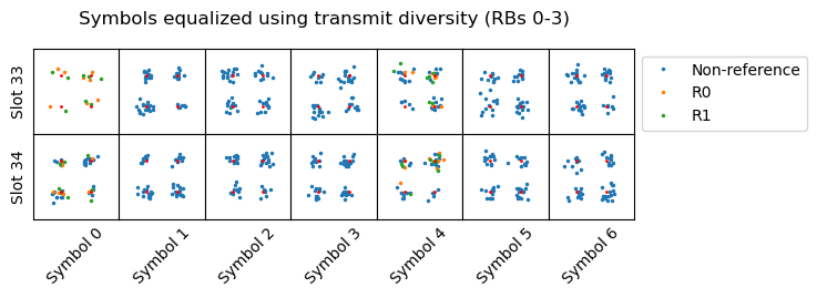
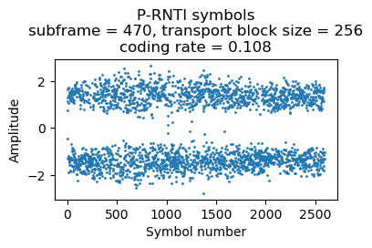
The constellation plots of the symbols for these transmissions are shown below. These are equalized for 2-port transmit diversity, because that is the transmission mechanism used by a 2-port eNB for the broadcast PDSCH transmissions (SI-RNTI, P-RNTI, RA-RNTI).

This is all the data we need to start decoding. The following sections cover the process step by step.
Extraction of the symbols and descrambling
The first step to decode the PDSCH is to extract the symbols from the resource elements in the PDSCH transmission to obtain the soft symbols for the codeword. Here I will assume a QPSK constellation, although I will show how to deal with QAM constellations below. The set of resource elements occupied by the PDSCH transmission is defined by several rules. In the frequency domain, the set of resource blocks is indicated in the DCI. In the time domain, the transmission occupies all the symbols of a subframe, minus the first 1, 2 or 3 symbols, which are reserved for the PDCCH and other control channels (according to the value of the CFI given by the PCFICH). As one can imagine, the resource elements that are occupied by the CRS (cell-specific reference signals) are not used by the PDSCH.
Additionally, the PDSCH also avoids the synchronization signals and the PBCH. This means that if the PDSCH transmission happens in a subframe where synchronization signals (subframes 0 and 5 of every radio frame) or the PBCH (subframe 0 of every radio frame) are present, then the central 6 resource blocks in those symbols in which the synchronization signals (both in subframes 0 and 5) and the PBCH (only in subframe 0) are present are avoided by the PDSCH. This needs to be taken into account when extracting the PDSCH symbols. In an cell which is sparsely utilized, such as the one in this recording, this situation rarely happens. In fact I’ve only found it once in the first 500 ms of the recording. In a heavily utilized cell it will happen more frequently.
The order in which the PDSCH resource elements are taken is in lexicographic order of time and frequency. First all the resource elements from the first symbol, in increasing order of frequency, then the resource elements of the second symbol, etc. In the case of a QPSK constellation, each QPSK symbol contributes two bits. The first is given by the real part, and the second by the imaginary part. Following all these rules, we can extract a list of soft symbols for the codeword.
The transmitted bits are scrambled using a pseudorandom sequence. The initialization of the pseudorandom sequence depends on the RNTI (which we know, since we have decoded the DCI), on the codeword number (up to two codewords can be transmitted simultaneously using spatial multiplexing), on the subframe number within the radio frame, and on the physical cell ID.
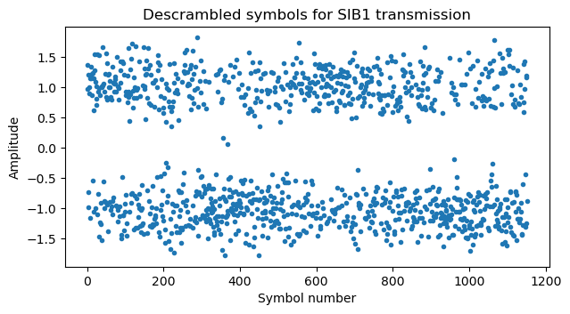
Undoing the scrambling, we obtain descrambled soft symbols for the SIB1 codeword. These are plotted here for the first of the two SIB1 transmissions that we’re using.
Rate matching
The PDSCH FEC is similar to the PBCH and PDCCH (see this post). The main difference is that an \(r = 1/3\) Turbo code is used instead of an \(r = 1/3\) convolutional code. The rate matching algorithm also has a few small differences.
Briefly speaking the whole FEC encoding process begins with a transport block, to which a CRC-24 is attached. If the resulting information block is longer than 6144 bits, which is the maximum codeword size supported by the Turbo encoder, then the information block is segmented into several codewords, and a CRC-24 computed with a different algorithm is attached to each codeword. I haven’t encountered any transport block that is long enough to be segmented in this recording, so I haven’t implemented this part of the process and I will be ignoring it in this post.
Additionally, in this code block segmentation step it might be necessary to add filler bits to pad it to one of the allowed Turbo codeword sizes, which are listed in Table 5.1.3-3 in TS 36.212. These filler bits have the value <NULL>, which has the special semantics that goes into the Turbo encoder input as if it was a zero, but its three corresponding Turbo encoder outputs are assigned the value <NULL>. Bits with <NULL> values, which are also produced during interleaving, are punctured during the rate matching process, so they never make it into the final codeword. All the transport blocks I have encountered match the size of a Turbo codeword, so I haven’t implemented this step either.
The Turbo encoder takes an input vector of length \(K\) and generates three output vectors of length \(K + 4\), where the 4 extra bits are a consequence of trellis termination. These output vectors are denoted by \(d^{(0)}\), \(d^{(1)}\), \(d^{(2)}\). The vector \(d^{(0)}\) corresponds to the systematic part of the encoder, so it is equal to the input vector, followed by 4 extra bits. The vectors \(d^{(1)}\) and \(d^{(2)}\) correspond to the outputs of the two constituent convolutional encoders that form the Turbo encoder.
The goal of the rate matching algorithm is to convert this input of length \(3(K + 4)\) into an output of the appropriate size to be modulated on the PDSCH transmission. This size is calculated as the number of resource elements occupied by the PDSCH transmission times the number of bits per constellation symbol (2 for QPSK, 4 for 16QAM, 6 for 64QAM, etc.). Recall that the number of resource elements occupied by a PDSCH transmission depends on the CFI (which determines how many symbols are reserved for the PDCCH), on the number of resource blocks allocated to the PDSCH transmission, on the number of antenna ports (since it determines the number of resource elements allocated to CRS, which the PDSCH avoids), and on whether the PDSCH allocation collides with synchronization signals and/or the PBCH. Rate matching performs puncturing and repetition of the Turbo codeword to obtain the required output size, thus realizing a coding rate which ranges between approximately between 0.076 and 0.86, even though the Turbo encoder always has a coding rate very close to 0.33.
The rate matching algorithm works as follows. First each of the input vectors \(d^{(0)}\), \(d^{(1)}\), \(d^{(2)}\) is interleaved. As in the case of the PBCH and PDCCH, the interleaver is based on a 32-column matrix in which the data is written by rows. Then the columns are permuted, and then the matrix is read by columns. If the length of the input \(d^{(j)}\) is not a multiple of 32, then it is padded with <NULL> bits at the beginning. This is basically the same as for the PBCH and PDCCH, except that the column permutation is different. There is also an additional twist in the PDSCH, because the vector \(d^{(2)}\) is processed slightly differently. Instead of writing the vector (plus any <NULL> padding) as such in the 32-column matrix, the vector and is padding are first circularly shifted by one place to the left before being written in the matrix. Then the process proceeds as for \(d^{(0)}\) and \(d^{(1)}\). Note that TS 36.212 explains the procedure for \(d^{(2)}\) differently, by giving the explicit formula for the interleaver permutation, but what I have described here is equivalent.
Applying interleaving to a Turbo encoder output is important to protect against burst errors. This is true even though the Turbo encoder uses interleaving internally (the second convolutional encoder operates on an interleaved version of the codeword). Section 7.4.4 in the CCSDS TM Synchronization and Channel Coding Green Book explains why. Even though this CCSDS book comes from spacecraft communications, the same principles are applicable to cellular communications.
The output of the interleaver consists of three vectors of size \(K_\Pi\), where \(K_\Pi\) is the smallest multiple of 32 that is greater or equal than \(K + 4\). The vectors are called \(\nu^{(0)}\), \(\nu^{(1)}\), \(\nu^{(2)}\), where each \(\nu^{(j)}\) is the interleaver output corresponding to \(d^{(j)}\). These three vectors are put together to form a vector of size \(K_w = 3 K_\Pi\). The way in which this is done is as follows: the first \(K_\Pi\) entries are the vector \(\nu^{(0)}\), which is the systematic part of the codeword. The remaining \(2 K_\Pi\) entries are formed by intertwining one bit from \(\nu^{(1)}\) and one bit from \(\nu^{(2)}\), instead of concatenating them. This is the “parity” part of the codeword. Note that this is different from what the convolutionally-encoded PBCH and PDCCH do. For the PBCH and PDCCH, the vectors \(\nu^{(1)}\) and \(\nu^{(2)}\) are concatenated instead of intertwined.
Now the bit selection algorithm obtains an \(E\) bit output (where \(E\) is the number of bits to be modulated in the PDSCH transmission) from this sequence of \(K_w\) bits. This is done similarly as for the PBCH and PDCCH. The sequence of \(K_w\) bits is treated as a circular buffer. The bit selection starts at a position \(k_0\) in this circular buffer, and advances along the buffer, skipping any <NULL> bits that it encounters, and copying any non-<NULL> bits to the output until it has obtained \(E\) bits. Depending on the values of \(E\) and \(K_w\) (which are related to the code rate), the bit selection might need to do several laps around the circular buffer, thus applying repetition coding. There is one twist in TS 36.212, which is that if \(K_w\) is very large (where “very large” is defined in terms of some complicated formulas involving the UE capabilities), then only the first \(N_{cb}\) bits of the \(K_w\) bit vector are used for the circular buffer. I haven’t encountered this situation in the recording, and have not implemented it.
In the bit selection of the PBCH and PDCCH, the starting point \(k_0\) is always zero. In the PDSCH, \(k_0\) depends on the redundancy version index, which is an integer between 0 and 3 (both included). The redundancy version index thus selects what part of the Turbo encoder output is transmitted (At least when the coding rate is much higher than 0.33. When the coding rate is much lower than 0.33, the bit selection algorithm needs to do several laps around the circular buffer, and all the output bits of the Turbo encoder are transmitted multiple times). The formula for \(k_0\) in Section 5.1.4.1.2 of TS 36.212 is\[k_0 = R^{TC}_{subblock}\cdot\left(2\cdot\left\lceil\frac{N_{cb}}{8R^{TC}_{subblock}}\right\rceil\cdot rv_{idx}+2\right).\]Here \(R^{TC}_{subblock} = K_\Pi / 32\) is the number of rows that were used in the matrix interleaver, \(N_{cb} = K_w = 3 K_\Pi\) unless \(K_w\) is very large as mentioned above, and \(rv_{idx}\) is the redundancy version index. When \(N_{cb} = K_w\), this expression can be simplified to\[k_0 = K_\Pi\cdot\left(\frac{3}{4}\cdot rv_{idx} + \frac{1}{16}\right).\]This is much easier to interpret. The length of the circular buffer is \(K_w = 3K_\Pi\), and there are 4 possible values for \(rv_{idx}\). These give 4 equally spaced positions covering the whole circular buffer because of the \(3K_\Pi \cdot rv_{idx}/4\) term. The additional subtlety is that these positions do not start at \(k_0 = 0\), but rather at \(k_0 = K_\Pi/16\).
Thus, for \(rv_{idx} = 0\), which is used for the first transmission of a codeword (and the only transmission whenever there are no retransmissions needed because the UE manages to decode the codeword with this first transmission). The rate matching skips the first two columns of the interleaver for the systematic part \(d^{(0)}\). Since the coding rate is always lower than 1 (otherwise decoding from a single redundancy version would be impossible), the bit selection algorithm for \(rv_{idx} = 0\) must continue into the parity part of the circular buffer, selecting at least some bits from \(d^{(1)}\) and \(d^{(2)}\). At least the first columns of the interleaver matrices for \(d^{(1)}\) and \(d^{(2)}\) will be taken. Note that these will correspond to different Turbo encoder steps, because of the circular shift that was applied to \(d^{(2)}\). Therefore, for high coding rate, \(rv_{idx} = 0\) punctures a few bits from the systematic part (one in every 16) and transmits some parity bits from \(d^{(1)}\) and \(d^{(2)}\) to compensate. If the coding rate gets lower and lower, then more and more parity bits from \(d^{(1)}\) and \(d^{(2)}\) get transmitted.
Now consider \(rv_{idx} = 1\), which would be used for a retransmission. This has \(k_0 = 13 K_\Pi / 16\), so the bit selection starts in column 26 of the interleaver matrix for \(d^{(0)}\). For high coding rate, only the last 6 columns of \(d^{(0)}\) are transmitted, followed somewhat more than 13 columns from \(d^{(1)}\) and \(d^{(2)}\). Thus, this redundancy version consists of a few systematic bits, and many parity bits. Since there is significant overlap with \(rv_{idx} = 0\), the receiver can use soft combining for the bits that appear in both codewords. Considering \(rv_{idx} = 2\), we see that \(k_0 = 37 K_\Pi/16\), so all the 32 columns of \(d^{(0)}\) have been skipped and the first 2.5 columns of \(d^{(1)}\) and \(d^{(2)}\) have been skipped too. Compared to \(rv_{idx} = 0\), the starting point \(rv_{idx} = 2\) is halfway along the circular buffer, or as far as it can get. If the coding rate is higher than approximately 0.66, then there will be no overlap in the bits selected by \(rv_{idx} = 0\) and \(rv_{idx} = 2\), because their starting points differ by \(3 K_\Pi / 2\), and the coding rate is approximately equal to \(K_\Pi / E\). Finally, \(rv_{idx} = 3\) has \(k_0 = 61K_\Pi/16\). This means that all of \(d^{(0)}\) plus the first 14.5 columns of \(d^{(1)}\) and \(d^{(2)}\) have been skipped. Therefore, this redundancy version transmits the last 17.5 columns of \(d^{(1)}\) and \(d^{(2)}\) and at least the first two columns of \(d^{(0)}\), which were skipped in \(rv_{idx} = 0\) (these are a total of 37 columns, so they are always transmitted, because 37 columns gives a coding rate of approximately 0.865, and the coding rate is never greater than this).
The above intuitive analysis of the effects of each redundancy version has been done with a high coding rate in mind. A similar analysis can be done for low coding rates. For these, the bit selection needs to do several laps around the circular buffer. For instance, for a coding rate of 0.1, the bit selection does 3 laps and a bit more around the buffer. Most of the bits are repeated 3 times in the output, but some of them (those at the position \(k_0\) and some of the following positions) are repeated 4 times. Therefore, the reasoning above for how the redundancy version affects \(k_0\) indicates which bits are “stronger” in the output because they are repeated one time more than the rest.
In many situations, the sequence in which redundancy versions are used if retransmissions are needed is 0, 2, 3, 1 (as mentioned above, this is always the case for the SIB1). The reasoning above justifies this choice. Assuming a high coding rate, redundancy version index 0 gives most of the systematic bits and a small amount of parity, which is enough to decode with a good SNR. If decoding fails, redundancy version index 2 gives a set of bits which is most disjoint with that of index 0, giving new information for the Turbo decoder and increasing the chances of decoding successfully. If another retransmission is needed, index 3 repeats some of the parity bits of index 2 and some of the systematic bits of index 0, as well as including the systematic that were missing in index 0. If decoding still fails, index 1 gives some more repetition of a mix of systematic and parity bits.
There is surely more detailed analysis of the performance of the Turbo decoder under different coding rates and combinations of different redundancy versions that has gone into the definitions of the rate matching algorithm in TS 36.212, but what I have mentioned here is probably good enough as simplified explanation.
Now onto the practical part. A receiver needs to run the rate matching algorithm in reverse by identifying which \(d^{(j)}_k\) bit corresponds to each of the descrambled soft symbols obtained from the PDSCH transmission. For this, it needs to know the redundancy version index and the transport block size (from which it can calculate all the sizes that derive from it, such as \(K_\Pi\)). This information is given in the DCI corresonding to the PDSCH transmission. My implementation of the rate matching algorithm is similar to the one I used for the PBCH and PDCCH. The algorithm takes as input the soft symbols from the transmission and produces an output dictionary where each index (j, k) is associated with the list of repetitions of the bit \(d^{(j)}_k\) in the transmission (some of these lists might be empty some particular \(d^{(j)}_k\) are not transmitted at all for this redundancy version, or it might have multiple repetitions of each \(d^{(j)}_k\) if the coding rate is low).
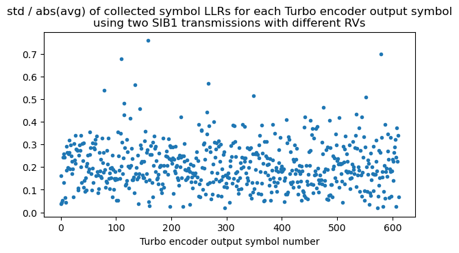
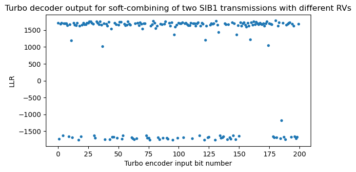
A good way to check that the implementation of the inversion of the rate matching algorithm is correct is to run it with a low coding rate PDSCH transmission and check that within each group of soft symbols corresponding to the same \(d^{(j)}_k\) all these soft symbols have the same sign (except for the occasional bit error). However, there are some things that this technique cannot check. For example, it doesn’t check at all whether \(k_0\) has been calculated correctly from \(rv_{idx}\). A consistency check that also involves the calculation of \(k_0\) is to use instead two PDSCH transmissions of the same transport block with different \(rv_{idx}\). The SIB1 is quite good to do this check, because it is transmitted with a low coding rate (broadcast PDSCH transmissions always use a low coding rate to ensure that all the UEs can decode them) and because there are 4 transmissions of the same data using different \(rv_{idx}\) values in a predictable way. Here I will use the two SIB1 transmissions that I have shown above, which have \(rv_{idx}\) equal to 2 and 3 respectively.
A way to do this check is to compute, within each group of soft symbols corresponding to the same \(d^{(j)}_k\), the standard deviation of the symbols divided by the absolute value of their average. This metric should be low if the grouping has been done correctly, as all the soft symbols within the group will have the same sign except when there are bit errors.
Since the Turbo decoder operates on LLRs, it is more natural to use LLRs at this point instead of soft symbols. Recall that the LLR for a BPSK or QPSK soft symbol is defined as\[L = -2\frac{y}{\sigma^2},\]where \(y\) is the received soft symbol (normalized to an amplitude of one) and \(\sigma\) is the noise standard deviation (on the real and on the imaginary part, so that the total noise power is \(2 \sigma^2)\)). Here I’m using the convention that a positive soft-symbol represents the bit 1, even though LTE prefers very much the opposite convention (in the LTE QPSK constellation, the point \((1 + 1j)/\sqrt{2}\) corresponds to the pair of bits 00, and so on). For the LLR, I’m using the most common convention that a positive LLR represents that the bit 0 is more likely. This is the reason why there is a minus sign in the formula. For all the decoding in this post I’m eyeballing a value of \(\sigma\), since this choice isn’t too critical to get good sensitivity in the Turbo decoder.
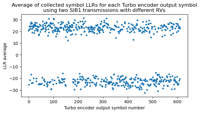
Here is a plot of the standard deviation divided by the absolute value of the average calculated using the two SIB1 transmissions with redundancy versions 2 and 3. This metric is relatively low, giving good confidence that the algorithm is correct. When I still had bugs in the implementation, the metric showed much higher values. This consistency check also verifies that descrambling has been performed correctly, because each repetition of the same \(d^{(j)}_k\) is scrambled with a different bit of the scrambling sequence.
We can also compute the average within each group of LLRs for the same \(d^{(j)}_k\) to check that all the entries in the group have the same sign and there is no cancellation. The following plot shows the average using these two SIB1 transmissions. The order on the x-axis is first all the \(d^{(0)}_k\), then all the \(d^{(1)}_k\), and finally all the \(d^{(2)}_k\), each ordered in increasing order of \(k\). Since the \(d^{(0)}_k\) are systematic bits, we can already see some features of the data. There is a prevalence of 0 bits (which have a positive LLR), and there is a segment of padding of all zeros at the end of the transport block, immediately before the CRC-24.
Turbo decoding
Once we have the LLRs grouped for each \(d^{(j)}_k\), we need to perform Turbo decoding. The first step is to perform soft-combining, to combine all the repetitions of the same \(d^{(j)}_k\) into a single value. When using LLRs, soft-combining is as easy as adding the LLRs of all the soft symbols corresponding to the same \(d^{(j)}_k\). If a certain \(d^{(j)}_k\) wasn’t transmitted at all, it gets the LLR zero.
The core of a Turbo decoder is the BCJR algorithm, which is used to obtain a MAP (maximum a posteriori) decode of each of the constituent convolutional codes. In each iteration of the Turbo decoder, BCJR is first used on the first convolutional code using extrinsic information generated from the second convolutional code (in the first iteration there is no such extrinsic information yet), and then BCJR is used on the second convolutional code using extrinsic information generated from the first convolutional code. The algorithm finishes after a fixed number of iterations (usually around 10 to 20 for best sensitivity) or when the CRC-24 of the current candidate codeword is correct, which allows an early termination to reduce the computational load. In my implementation I’m doing a fixed number of 10 iterations for simplicity.
I have adapted the BCJR implementation that I first wrote for Voyager-1, and I have followed Algorithms 5.1 and 4.2 in Sarah Johnson’s book quite closely. The implementation is not fast at all, but it is easy to read. The only precaution that I’ve had to take is to clip the LLRs to a minimum value of -512 and a maximum value of 512 (which are huge LLRs, by all means), since otherwise I run into numerical problems when computing the function \(\log(1 + e^{\pm L})\) for very large LLRs \(L\) (the value of \(\log(1 + e^{L})\) should be very close to \(L\) when \(L > 0\) is large, but the calculation of \(e^{L}\) gives infinity in double precision).
The trellis termination of the LTE Turbo encoder is somewhat peculiar, since it is different from how other Turbo codes, such as the CCSDS code described in the TM Synchronization and Channel Coding Blue Book, are terminated. In order to terminate a Turbo code, the shift registers in its convolutional encoders need to be driven to zero by inserting the appropriate termination bits after the message to be encoded has been inserted. The termination bits are such that they cause a zero to be inserted into the shift register of the encoder, and thus are the same as the feedback bits, so as to cancel the feedback and get a zero at the shift register input. After inserting \(k\) termination bits, where \(k\) is the number of stages in the shift register (\(k = 3\) for the LTE Turbo code), the shift register contains all zeros. This termination process is usually shown in the diagram of a Turbo encoder by some switches that get engaged during the termination. For instance, TS 36.212 shows some dotted lines and switches.
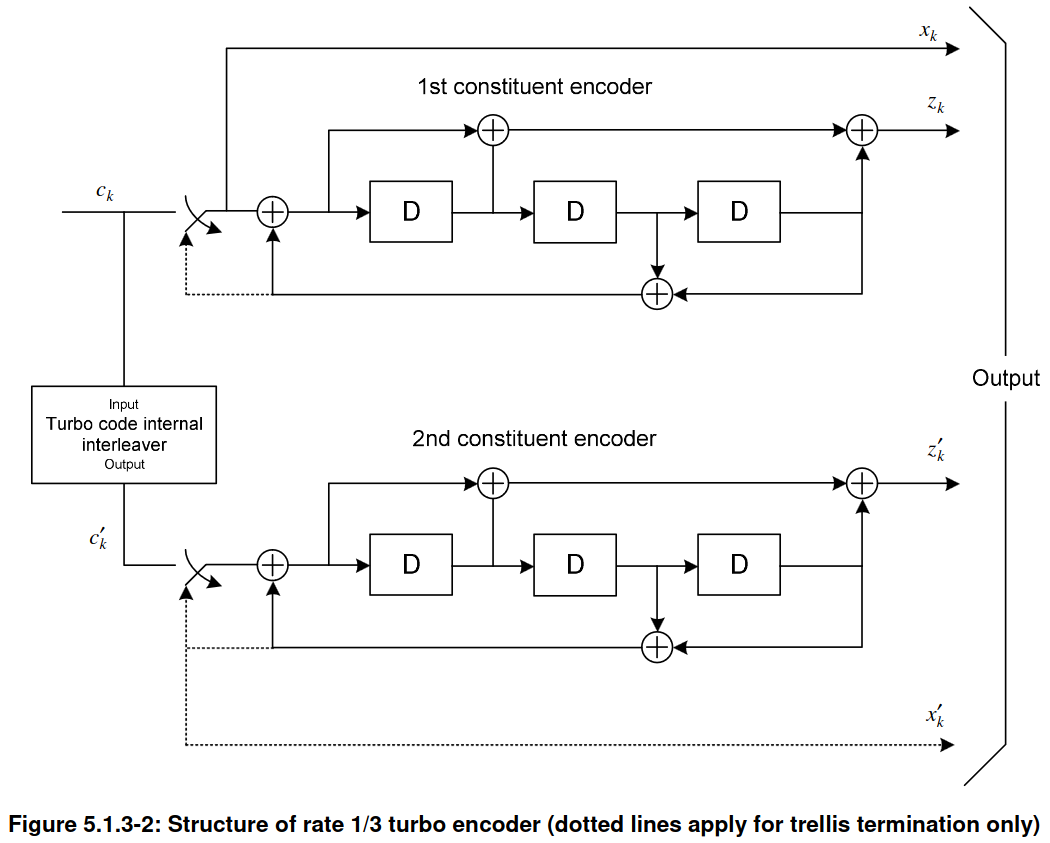
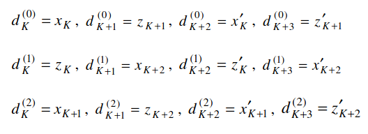
When the termination process begins, the contents of the two convolutional encoders are generally different, because they have been encoding different inputs (the second convolutional encoder operates on an interleaved version of the input). Therefore, the termination bits for each encoder are different. An encoder such as the CCSDS Turbo encoder transmits as systematic bits the termination bits of the first encoder and does not pass to the output the termination bits for the second encoder. In contrast, the LTE Turbo encoder is converted into a rate 1/4 encoder temporarily during termination by generating an additional output containing the termination bits for the second encoder. This is the \(x_k’\) shown above with a dotted line. For the termination, \(k = 3\) bits need to be inserted in the convolutional encoders, but for each of these bits, 4 output bits are produced instead of 3. Thus, the encoder produces a total of 12 output bits during termination. These are shuffled as indicated by the equations below, and each \(d^{(j)}\) is extended with 4 bits.
This peculiarity of the termination needs to be taken into account in the Turbo decoder implementation. For the non-termination trellis stages, the systematic bits of the first encoder come from the \(d^{(0)}\) bits, and the systematic bits of the second encoder are the \(d^{(0)}\) permuted according to the internal Turbo encoder permutation. However, for the termination trellis stages, the systematic bits of each of the two encoders are \(x_K, x_{K+1}, x_{K+2}\) and \(x_K’, x_{K+1}’, x_{K+2}’\), and must be taken from the \(d^{(j)}_k\) by using the formulas given above. A similar thing happens for the non-systematic bits.
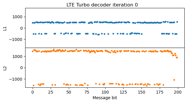
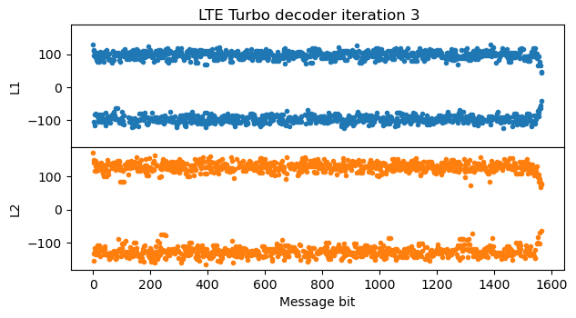
A good way to check that the Turbo decoder implementation is working and to debug any possible problems is to plot the evolution of the decoder state through each of the iterations. The most important part of the state is the LLRs \(L_1\) and \(L_2\) obtained by the two BCJR decoders. The LLR \(L_1\) gives directly the LLRs for the message bits, while \(L_2\) gives the LLRs for the interleaved version of the message. The output of the Turbo decoder is the \(L_2\) from the last iteration with the inverse interleaver permutation applied, so that it refers to the message bits in the correct order.
The following figure shows the values of \(L_1\) and \(L_2\) after the first iteration. In this case, the SNR at the input of the Turbo encoder is already very good and there are no bit errors or punctured bits, so a single pass of the BCJR decoder for the first convolutional encoder is enough to give very high LLRs in \(L_1\), shown in blue. The pass of the BCJR decoder for the second convolutional encoder using the extrinsic information generated by the first BCJR decoder is shown in orange. The LLRs grow even more, but they drop somewhat at the end of the message. The reason is that there is no extrinsic information for the trellis termination bits.
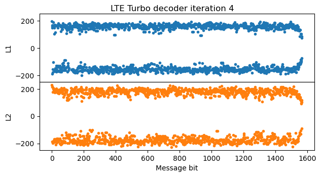
In the next iteration of the Turbo decoder, \(L_1\) looks quite similar to the \(L_2\) of the first iteration (except for fact that \(L_1\) and \(L_2\) are related by a permutation, which is visible by the parts where the LLRs are positive, representing zeros in the message). The LLRs don’t grow anymore, because I’m clipping the extrinsic information LLRs to the range [-512, 512] to avoid numerical problems. All the remaining iterations of the Turbo decoder look very similar to this second iteration.
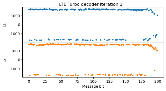
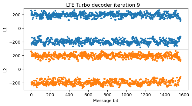
The final output of the Turbo decoder is obtained as a permutation of the \(L_2\) from the last iteration. We can see how the bits with smaller LLR at the end of the message get redistributed by the permutation.
The message bits are obtained by slicing the Turbo decoder output. A positive LLR corresponds to the bit 0. The last 24 bits of the message are a CRC-24. We can now check the CRC-24 to make sure that the decoding is implemented correctly. Other tests that we can do is to decode each of the redundancy versions of the SIB1 separately, or to decode the soft-combining of other combinations of redundancy versions.
Decoding other PDSCH transmissions
The same PDSCH decoder implementation that I have written for the SIB1 can be used for any QPSK PDSCH transmission whose transport block is not so large that it needs to be segmented into several code blocks. I have put this into practice by decoding all the PDSCH transmissions in the first 500 ms of the recording, except those that use two-codeword TM4 (as I explained in my previous post, a receiver with a single antenna cannot separate the two codewords).
To do this, I have continued using the same technique of my post about the PDCCH to find by hand for each subframe which DCIs are present in the PDCCH and what CCEs they have allocated, without knowing the RNTIs that are used by the cell. In the PDCCH post I did this for the first 50 ms of the recording. Now I have continued this process until the 500 ms mark, discovering other C-RNTIs that are active, and some interesting transmissions (such as a 64QAM transmission that we will analyse below).
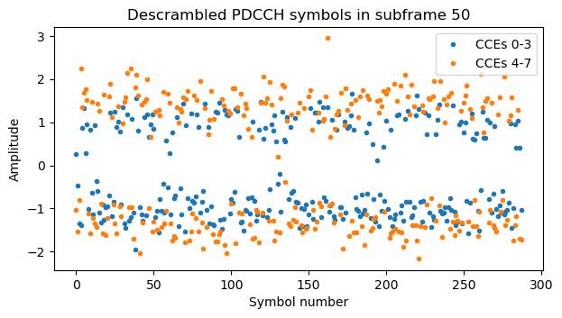
Something I have observed, related to the topic of downlink power allocation that I treated in the post about TM4 is that sometimes the PDCCH tranmissions use different power, even in the same subframe. For instance, this plot shows the symbols for two DCIs with aggregation level 4 in the same subframe. It seems that one of them uses amplitude 1, and the other uses amplitude \(\sqrt{2}\). I haven’t found any mention about the possibility of using a different amplitude for each PDCCH transmission in the 3GPP documents.
In the next sections I look at the contents of each PDSCH transmission, classified by its type, as given by the RNTI.
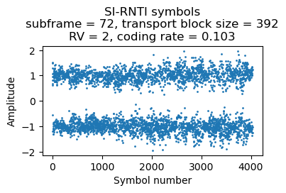
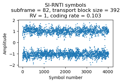
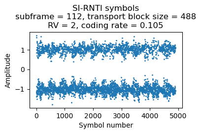
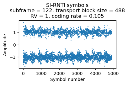
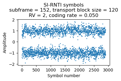
SI-RNTI
The SI-RNTI 0xffff contains the cell system information, which is transmitted in blocks such as the SIB1, SIB2, etc. We have already seen that there is a SIB1 transmission every 20 ms. Each four consecutive transmissions are retransmissions of the same SIB1 using different redundancy versions. In principle, the SIB1 contents could change with a granularity of 80 ms, but since the system information changes quite infrequently, in the recording all the SIB1 transmissions contain the same data.
This data is parsed using the ASN.1 definitions that can be found in TS 36.331. These are scattered through the PDF and Word documents, which is rather inconvenient. I have found that the OpenAirInterface5G project has files with the definitions extracted from the document using a Perl script, so I’m using one of these files. I already used the asn1tools Python package to parse the MIB contained in the PBCH. However, when doing this, I had wrongly set the encoding rules to PER instead of uPER. Since the MIB doesn’t contain any field that can be encoded to a length that is not a multiple of 8 bits, PER and uPER rules are the same for it. However, when treating other LTE messages the difference between PER and uPER is important. The rules that must be used are always uPER.
All the transport blocks transmitted with the SI-RNTI must be parsed with the BCCH-DL-SCH-Message, since they are messages from the BCCH (broadcast control channel). In the case of the SIB1, its contents are the following.
{'message': ('c1',
  ('systemInformationBlockType1',
   {'cellAccessRelatedInfo': {'plmn-IdentityList': [{'plmn-Identity': {'mcc': [2,
         1,
         4],
        'mnc': [0, 1]},
       'cellReservedForOperatorUse': 'notReserved'}],
     'trackingAreaCode': (b'\x01\x16', 16),
     'cellIdentity': (b'F\x07@p', 28),
     'cellBarred': 'notBarred',
     'intraFreqReselection': 'allowed',
     'csg-Indication': False},
    'cellSelectionInfo': {'q-RxLevMin': -64},
    'freqBandIndicator': 20,
    'schedulingInfoList': [{'si-Periodicity': 'rf16',
      'sib-MappingInfo': ['sibType3']},
     {'si-Periodicity': 'rf32', 'sib-MappingInfo': ['sibType5']},
     {'si-Periodicity': 'rf64', 'sib-MappingInfo': ['sibType6']}],
    'si-WindowLength': 'ms40',
    'systemInfoValueTag': 11,
    'nonCriticalExtension': {'nonCriticalExtension': {'cellSelectionInfo-v920': {'q-QualMin-r9': -18}}}}))}
The PLMN is 21401, which is assigned to Vodafone (see this database). This is to be expected, since the eNB I recorded is indeed from Vodafone. The TAC and cell ID, converted to decimal, are respectively 278 and 73430023. Unfortunately this particular cell doesn’t appear in OpenCellID nor in CellMapper, but other cells around the same area have the same TAC and a similar cell ID. We can also see that the frequencyBandIndicator is 20. Indeed this is a recording of a cell in the band B20.
The SIB1 lists which other SIBs are sent by the cell, and the periodicity with which they appear. The SIBs that are active are SIB3, SIB5 and SIB6, and also SIB2, because it is always implicitly present in the first entry of the schedulingInfoList. SIB6 is only transmitted every 64 radio frames, or 640 ms, but luckily for us, the first SFN in the recording is 313. Since SFN 320 is divisible by 64, the SIB6 transmission must happen at some point between this frame and 40 ms later (the value given by the si-WindowLength), so we are guaranteed to see a SIB6 quite close to the beginning of the recording.
The SIB2 and SIB3 are transmitted together in the same transport block. The SIB2/SIB3 and the SIB5 are transmitted twice with a spacing of 10 ms and redundancy versions 2 and 1. The SIB6 is only transmitted once with redundancy version 2.
In this cell, SI-RNTI transmissions are always allocated to the lower resource blocks of the cell. The number of resource blocks depends on the length of the data, and is chosen to give a particular coding rate. The SIB1 transmissions use 4 RBs, which gives a coding rate of 0.17 or 0.19 depending on the CFI. The SIB2/SIB3 transmissions use 14 RBs, for a coding rate of 0.1. The SIB5 transmissions use 17 RBs, which also gives a coding rate of 0.1. The SIB6 transmission uses 11 RBs, yieling a coding rate of 0.05. I guess this choice of coding rates is reasonable because the SIB1 is repeated 4 times, the SIB2/SIB3 and SIB5 are repeated 2 times, and the SIB6 is only sent once. So the coding rate for a UE that combines all the available repetitions would be around 0.05 in all the cases. This coding rate is slightly below the minimum of 0.076 that can be used to transmit user data, ensuring that all the UEs that can receive the cell with enough SNR to stay connected can also decode all the SIBs.
Here are the soft symbols for the first two SIB2/SIB3 transmissions.
The contents of the SIB2/SIB3 are as follows:
{'message': ('c1',
  ('systemInformation',
   {'criticalExtensions': ('systemInformation-r8',
     {'sib-TypeAndInfo': [('sib2',
        {'ac-BarringInfo': {'ac-BarringForEmergency': False},
         'radioResourceConfigCommon': {'rach-ConfigCommon': {'preambleInfo': {'numberOfRA-Preambles': 'n28',
            'preamblesGroupAConfig': {'sizeOfRA-PreamblesGroupA': 'n16',
             'messageSizeGroupA': 'b56',
             'messagePowerOffsetGroupB': 'dB10'}},
           'powerRampingParameters': {'powerRampingStep': 'dB2',
            'preambleInitialReceivedTargetPower': 'dBm-104'},
           'ra-SupervisionInfo': {'preambleTransMax': 'n10',
            'ra-ResponseWindowSize': 'sf10',
            'mac-ContentionResolutionTimer': 'sf64'},
           'maxHARQ-Msg3Tx': 5},
          'bcch-Config': {'modificationPeriodCoeff': 'n4'},
          'pcch-Config': {'defaultPagingCycle': 'rf64', 'nB': 'oneT'},
          'prach-Config': {'rootSequenceIndex': 176,
           'prach-ConfigInfo': {'prach-ConfigIndex': 19,
            'highSpeedFlag': False,
            'zeroCorrelationZoneConfig': 14,
            'prach-FreqOffset': 7}},
          'pdsch-ConfigCommon': {'referenceSignalPower': 15, 'p-b': 1},
          'pusch-ConfigCommon': {'pusch-ConfigBasic': {'n-SB': 4,
            'hoppingMode': 'interSubFrame',
            'pusch-HoppingOffset': 22,
            'enable64QAM': True},
           'ul-ReferenceSignalsPUSCH': {'groupHoppingEnabled': False,
            'groupAssignmentPUSCH': 0,
            'sequenceHoppingEnabled': False,
            'cyclicShift': 0}},
          'pucch-ConfigCommon': {'deltaPUCCH-Shift': 'ds1',
           'nRB-CQI': 3,
           'nCS-AN': 0,
           'n1PUCCH-AN': 54},
          'soundingRS-UL-ConfigCommon': ('release', None),
          'uplinkPowerControlCommon': {'p0-NominalPUSCH': -67,
           'alpha': 'al07',
           'p0-NominalPUCCH': -115,
           'deltaFList-PUCCH': {'deltaF-PUCCH-Format1': 'deltaF0',
            'deltaF-PUCCH-Format1b': 'deltaF3',
            'deltaF-PUCCH-Format2': 'deltaF1',
            'deltaF-PUCCH-Format2a': 'deltaF2',
            'deltaF-PUCCH-Format2b': 'deltaF2'},
           'deltaPreambleMsg3': 4},
          'ul-CyclicPrefixLength': 'len1',
          'pusch-ConfigCommon-v1270': {'enable64QAM-v1270': 'true'}},
         'ue-TimersAndConstants': {'t300': 'ms1000',
          't301': 'ms200',
          't310': 'ms1000',
          'n310': 'n10',
          't311': 'ms10000',
          'n311': 'n1'},
         'freqInfo': {'ul-Bandwidth': 'n50', 'additionalSpectrumEmission': 1},
         'timeAlignmentTimerCommon': 'infinity',
         'ac-BarringSkipForMMTELVoice-r12': 'true',
         'ac-BarringSkipForMMTELVideo-r12': 'true',
         'ac-BarringSkipForSMS-r12': 'true',
         'voiceServiceCauseIndication-r12': 'true'}),
       ('sib3',
        {'cellReselectionInfoCommon': {'q-Hyst': 'dB4',
          'speedStateReselectionPars': {'mobilityStateParameters': {'t-Evaluation': 's60',
            't-HystNormal': 's30',
            'n-CellChangeMedium': 4,
            'n-CellChangeHigh': 8},
           'q-HystSF': {'sf-Medium': 'dB0', 'sf-High': 'dB0'}}},
         'cellReselectionServingFreqInfo': {'s-NonIntraSearch': 6,
          'threshServingLow': 5,
          'cellReselectionPriority': 4},
         'intraFreqCellReselectionInfo': {'q-RxLevMin': -64,
          's-IntraSearch': 31,
          'presenceAntennaPort1': False,
          'neighCellConfig': (b'@', 2),
          't-ReselectionEUTRA': 1,
          't-ReselectionEUTRA-SF': {'sf-Medium': 'lDot0',
           'sf-High': 'oDot75'}}})]})}))}
The SIB2 contains some interesting information about the physical layer. The pdsch-ConfigCommon says that the p-b parameter is 1. As I mentioned in the section about downlink power alloction my post about TM4, for a two-port cell this means that all the PDSCH resource elements have the same power regardless of whether they occur on a symbol which contains CRS. It also says that the CRS power is 15 dBm (per subcarrier, that is). A transmission with all the 600 subcarriers of this 10 MHz cell utilized at the same power as the CRS would have 42.8 dBm, or 19W, so this sounds about right. The SIB3 contains cell re-selection parameters.
The following shows the soft symbols for two repetitions of the SIB5.
The SIB5 contains inter-frequency neighbouring cells, which are nearby cells in other frequencies. The dl-CarrierFreq parameter gives the downlink EARFCN, and the allowedMeasBandwidth gives the bandwidth of the cell in resource blocks: 100 RBs is a 20 MHz cell, 50 RBs is a 10 MHz cell, and 25 RBs is a 5 MHz cell. Using an EARFCN calculator, we get that the cells listed here have the following frequencies, which we can check in the frequency allocations of cell operators in Spain:
- 1835.1 MHz, 20 MHz bandwidth (Vodafone allocation in B3)
- 2670 MHz, 20 MHz bandwidth (Vodafone allocation in B7)
- 2150.1 MHz, 10 MHz bandwidth (Vodafone allocation in B1, which interestingly in the wiki shows as a 15 MHz allocation 2140-2155 MHz).
- 2152.6 MHz, 5 MHz bandwidth (this seems to be part of the same 15 MHz Vodafone allocation in B1, though it overlaps with the previous cell).
- 952.4 MHz, 5 MHz bandwidth (this is part of the Vodafone B8 allocation, although in the wiki it shows as the 10 MHz block 949.9-959.9 MHz, so this is only the lower 5 MHz of the block).
{'message': ('c1',
  ('systemInformation',
   {'criticalExtensions': ('systemInformation-r8',
     {'sib-TypeAndInfo': [('sib5',
        {'interFreqCarrierFreqList': [{'dl-CarrierFreq': 1501,
           'q-RxLevMin': -64,
           't-ReselectionEUTRA': 2,
           'threshX-High': 5,
           'threshX-Low': 5,
           'allowedMeasBandwidth': 'mbw100',
           'presenceAntennaPort1': False,
           'cellReselectionPriority': 6,
           'neighCellConfig': (b'@', 2),
           'q-OffsetFreq': 'dB0',
           'q-QualMin-r9': -18},
          {'dl-CarrierFreq': 3250,
           'q-RxLevMin': -64,
           't-ReselectionEUTRA': 2,
           'threshX-High': 8,
           'threshX-Low': 8,
           'allowedMeasBandwidth': 'mbw100',
           'presenceAntennaPort1': False,
           'cellReselectionPriority': 6,
           'neighCellConfig': (b'@', 2),
           'q-OffsetFreq': 'dB0',
           'q-QualMin-r9': -18},
          {'dl-CarrierFreq': 401,
           'q-RxLevMin': -64,
           't-ReselectionEUTRA': 2,
           'threshX-High': 5,
           'threshX-Low': 5,
           'allowedMeasBandwidth': 'mbw50',
           'presenceAntennaPort1': False,
           'cellReselectionPriority': 5,
           'neighCellConfig': (b'@', 2),
           'q-OffsetFreq': 'dB0',
           'q-QualMin-r9': -18},
          {'dl-CarrierFreq': 426,
           'q-RxLevMin': -64,
           't-ReselectionEUTRA': 2,
           'threshX-High': 6,
           'threshX-Low': 5,
           'allowedMeasBandwidth': 'mbw25',
           'presenceAntennaPort1': False,
           'cellReselectionPriority': 3,
           'neighCellConfig': (b'@', 2),
           'q-OffsetFreq': 'dB0',
           'q-QualMin-r9': -18},
          {'dl-CarrierFreq': 3724,
           'q-RxLevMin': -64,
           't-ReselectionEUTRA': 2,
           'threshX-High': 7,
           'threshX-Low': 6,
           'allowedMeasBandwidth': 'mbw25',
           'presenceAntennaPort1': False,
           'cellReselectionPriority': 3,
           'neighCellConfig': (b'@', 2),
           'q-OffsetFreq': 'dB0',
           'q-QualMin-r9': -18}]})]})}))}
Interestingly all these entries have presenceAntennaPort1 set to false, which means that some cells might use a single antenna port.
Finally, the following plot shows the soft symbols of the SIB6 transmission.
The SIB6 contains information about neighbouring UMTS (3G) cells. We can use an ARFCN calculator to obtain the corresponding frequencies. These are 952.4 MHz (Vodafone B8 allocation) and 2142.6 MHz (which belongs to the Vodafone B1 allocation).
P-RNTI
The P-RNTI is using for paging UEs, which is the way of notifying UEs that are in idle mode using discontinuous reception (DRX). These UEs only monitor the PCCH (paging control channel, which is transmitted in the PDSCH using the P-RNTI) periodically to check if the network has something for them.
The frames and subframes in which the PCCH can be transmitted are defined in Section 7 in TS 36.304. The configuration depends on the nB parameter, which is transmitted in the pcch-Config of the SIB2. For this cell, nB has the value oneT, which means that the variable nB has the value T (which stands for the UE DRX cycle) wherever it appears in the equations. Since Ns = max(1, nB/T), for this cell Ns = 1, and we see using the table in Section 7.2 that the PCCH can only be transmitted in subframe 9. In fact this is what happens in the recording. Subframe 9 in most of the radio frames have a PCCH transmission. There are a few radio frames with no PCCH transmissions, since there are no paging messages to send in those particular frames.
Moreover, applying other equations from Section 7 in TS 36.304 we see that the SFN in which a paging message addressed to a particular UE can be transmitted is equal to the UE IMSI mod 1024 and mod T. The IMSI (international mobile subscriber identity) is the unique ID of a UE, but we don’t have access to the IMSIs. These are sent as rarely as possible to prevent tracking by eavesdroppers. Instead, usually the TMSI (temporary mobile subscriber identity) is transmitted in place of the IMSI. The TMSI is assigned pseudorandomly to the UE when it connects to the network. The paging messages transmitted by the PCCH contain TMSIs. We don’t know the mapping between IMSIs and TMSIs, so we can’t check that the paging messages have been transmitted in the appropriate SFN according to the rules in TS 36.304, but at least we can see that each PCCH transmission in the 500 ms I have decoded is always addressed to different TMSIs (a TMSI never repeats in such two transmissions). This cell has a defaultPagingCycle equal to rf64 (64 radio frames, or 640 ms) in the pcch-Config in SIB2. This is what gives the value of T unless it has been overridden for a particular UE by higher layers. Therefore, a paging message to a UE would only repeat after 640 ms.
Something interesting about the PCCH is that the size of the PCCH-Message that it transmits depends on the number of PagingRecords that are present. For the transmissions that I have decoded, this ranges between 1 and 5 (and most frequently it is 1). This cell always allocates the lower resource blocks to transmit the P-RNTI, but the amount of resource blocks used depends on the length of the message and it is chosen to give a coding rate close to 0.1.
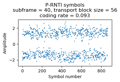
As an example, here are the soft symbols of a P-RNTI transmission containing one paging record. This uses 3 RBs.
The parsed data is
{'message': ('c1',
  ('paging',
   {'pagingRecordList': [{'ue-Identity': ('s-TMSI',
       {'mmec': (b'\xb0', 8), 'm-TMSI': (b'\xd1F\xef~', 32)}),
      'cn-Domain': 'ps'}]}))}
A P-RNTI transmission with 2 paging records uses 4 RBs (others can use 5 RBs, depending on the CFI).
{'message': ('c1',
  ('paging',
   {'pagingRecordList': [{'ue-Identity': ('s-TMSI',
       {'mmec': (b'\xd0', 8), 'm-TMSI': (b'\xc8\xf1F\xb6', 32)}),
      'cn-Domain': 'ps'},
     {'ue-Identity': ('s-TMSI',
       {'mmec': (b'\xe8', 8), 'm-TMSI': (b'\xf9\x8b\xbc\xbc', 32)}),
      'cn-Domain': 'ps'}]}))}
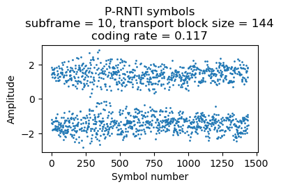
Here is a transmission with 3 paging records, which uses 5 RBs (others can use 6 RBs, depending on the CFI).
{'message': ('c1',
  ('paging',
   {'pagingRecordList': [{'ue-Identity': ('s-TMSI',
       {'mmec': (b'\xd0', 8), 'm-TMSI': (b'\xca\xd1\xb2J', 32)}),
      'cn-Domain': 'ps'},
     {'ue-Identity': ('s-TMSI',
       {'mmec': (b'\xc8', 8), 'm-TMSI': (b'\xfdO\xb9R', 32)}),
      'cn-Domain': 'ps'},
     {'ue-Identity': ('s-TMSI',
       {'mmec': (b'\xc8', 8), 'm-TMSI': (b'\xdb7\x08q', 32)}),
      'cn-Domain': 'ps'}]}))}
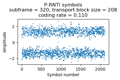
Here is a transmission with 4 paging records. It uses 8 RBs.
{'message': ('c1',
  ('paging',
   {'pagingRecordList': [{'ue-Identity': ('s-TMSI',
       {'mmec': (b'\xb8', 8), 'm-TMSI': (b'\xf3dF\xa0', 32)}),
      'cn-Domain': 'ps'},
     {'ue-Identity': ('s-TMSI',
       {'mmec': (b'\xc0', 8), 'm-TMSI': (b'\xc4\x1eN{', 32)}),
      'cn-Domain': 'ps'},
     {'ue-Identity': ('s-TMSI',
       {'mmec': (b'\xc0', 8), 'm-TMSI': (b'\xda\x1a\xa5\x0b', 32)}),
      'cn-Domain': 'ps'},
     {'ue-Identity': ('s-TMSI',
       {'mmec': (b'\xc8', 8), 'm-TMSI': (b'\xfd\x0b\x94\x02', 32)}),
      'cn-Domain': 'ps'}]}))}
Finally, here is a transmission with 5 paging records, which uses 9 RBs.
{'message': ('c1',
  ('paging',
   {'pagingRecordList': [{'ue-Identity': ('s-TMSI',
       {'mmec': (b'\xd0', 8), 'm-TMSI': (b'\xf3\xdb\xb8J', 32)}),
      'cn-Domain': 'ps'},
     {'ue-Identity': ('s-TMSI',
       {'mmec': (b'\xe8', 8), 'm-TMSI': (b'\xfe\xa5\xca\r', 32)}),
      'cn-Domain': 'ps'},
     {'ue-Identity': ('s-TMSI',
       {'mmec': (b'\xc0', 8), 'm-TMSI': (b'\xd4\x8d\xe2\x05', 32)}),
      'cn-Domain': 'ps'},
     {'ue-Identity': ('s-TMSI',
       {'mmec': (b'\xc0', 8), 'm-TMSI': (b'\xfa\x0b\x82\xa8', 32)}),
      'cn-Domain': 'ps'},
     {'ue-Identity': ('s-TMSI',
       {'mmec': (b'\xe8', 8), 'm-TMSI': (b'\xe9\xe6H6', 32)}),
      'cn-Domain': 'ps'}]}))}
Plots and decoded data for all the P-RNTI transmissions can be seen in the Jupyter notebook.
Interestingly it looks like the P-RNTI transmissions are sent with more power than the SI-RNTI transmissions. The amplitude of the soft symbols in these plots looks to be closer to \(\sqrt{2}\) than to one. Compare this with the plots of the SI-RNTI in the previous section, in which the amplitude of the soft symbols is close to one.
C-RNTI
C-RNTI stands for cell RNTI. This is used for PDSCH transmissions addressed to an individual UE. Decoding C-RNTI transmissions is more interesting than decoding SI-RNTI and P-RNTI transmissions, because there is much more variety in the configuration and specific details of each transmission.
For a two-port cell such as this one, all the broadcast transmissions, including the SI-RNTI and P-RNTI are sent using transmit diversity. Transmissions to a single UE can employ other transmission methods that better target that UE. All the C-RNTI transmissions that I’ve seen in this recording use TM4 (closed-loop spatial multiplexing). TM4 can transmit either one or two codewords at the same time (this is what spatial multiplexing means). For some UEs, only one codeword is used, while for others the transmissions are predominantly sent with two codewords. This probably depends on the number of antenna ports that the UE has reported to have, since two-codeword TM4 needs 2×2 MIMO. Occassionally one of the UEs that use two-codeword TM4 fails to decode one of the codewords, and only the codeword that was missed is retransmitted with single-codeword TM4. In this way, we can decode some transmissions for these UEs, since with a single-antenna recording we cannot decode two-codeword transmissions.
Here is a summary of the UEs that appear in the recording, classified by their C-RNTI, showing how the PDSCH transmissions addressed to each UE look like. Plots for all the transmissions are available in the Jupyter notebook.
C-RNTI 0xc33c
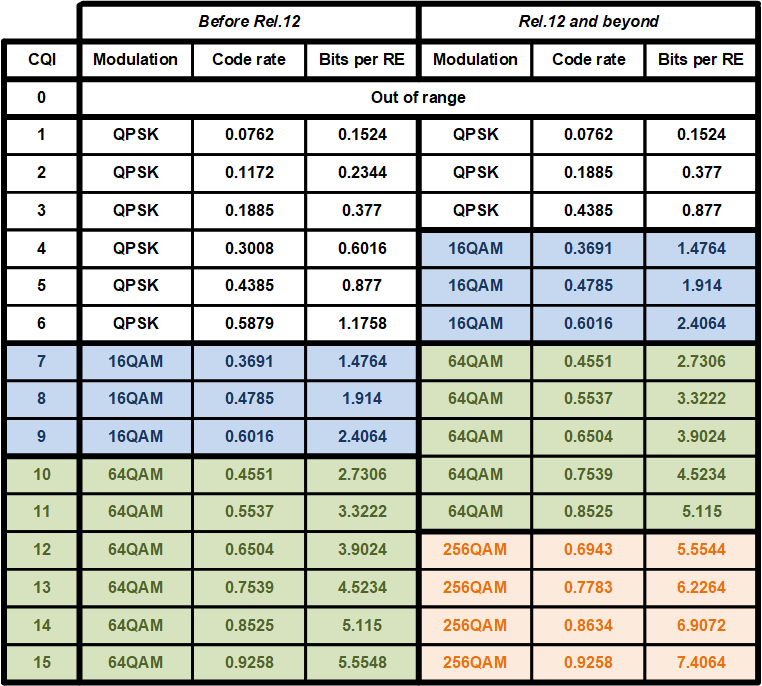
Data is sent to this UE in a very regular manner. A transmission is sent approximately every 20 ms (more precisely, the transmissions are spaced by 19, 20 or 21 subframes). Most transmissions use a transport block size of 424 bits and resource blocks 36-47 (12 RBs), giving a coding rate of 0.13. Looking at the following table, which gives the correspondence between CQI and coding rate, we see that most likely this UE is reporting CQI 2.
The other transmissions have slightly different transport block sizes, RB allocations and coding rates. As we will see later, the difference in transport block size is only caused by a difference in padding in the MAC PDUs. All the MAC PDUs transmitted to this UE actually carry a 39 byte SDU.
All the transmissions use redundancy version 0. There are no retransmissions. Since the spacing between transmissions is larger than 8 ms, all of them use HARQ process 7, since there is enough time for the HARQ ACK/NACK to come back (briefly speaking, the HARQ information in LTE has a round-trip time of 8 ms, so a different HARQ process is used to send transmissions spaced by less than 8 ms, because by the time that the second transmission needs to be sent, the ACK/NACK for the first transmission hasn’t come back yet). All the transmissions use precoding matrix number 3.
Here are the DCI and the soft symbols corresponding to the first of these transmissions.
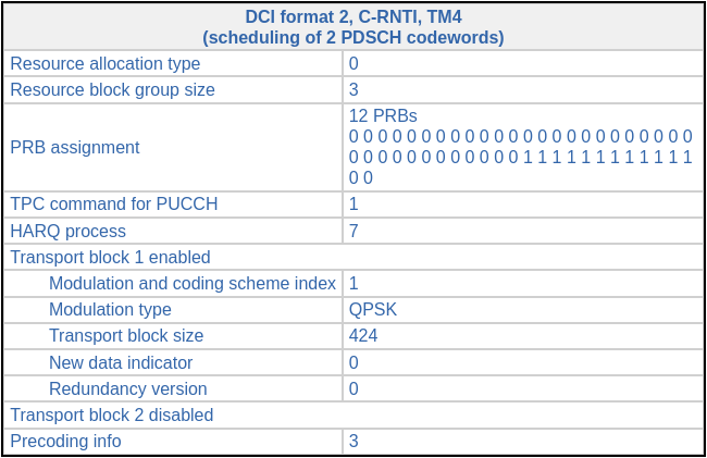
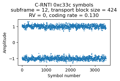
The decoded data in hex (minus the CRC-24) for this transmission is:
25271f00f985f1ae4e9dea164ad9052323091221050e5a80dc6dbb5d63cbced8b56dbe4262102125504385c71d4b2a45457482aeeb
As we will see below, the transport block for C-RNTI transmissions is a MAC PDU. It should be parsed as indicated in this ShareTechnote page to obtain the SDUs and the control information that are carried in the MAC PDU.
C-RNTI 0xced8
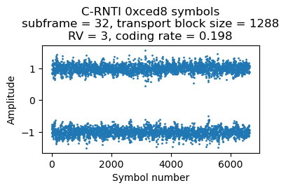
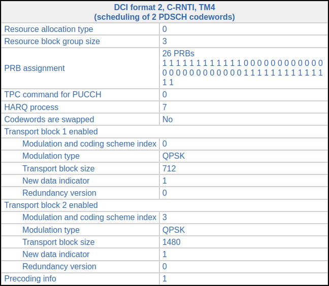
Most of the transmissions to this UE use two-codeword TM4. Occasionally the UE misses one of the codewords, and it is then retransmitted in single-codeword TM4. The first time that this happens is in subframe 32 (using a subframe numbering that starts at the beginning of the recording, without any consideration for the radio frame structure and SFN). In subframe 18 there was the following transmission.

Then, in subframe 32 (14 ms later) there is the following DCI, indicating a retransmission of the first codeword, this time using redundancy version 3 and a slightly different resource block allocation. We know that this is a retransmission because the new data indicator hasn’t toggled with respect to the previous DCI in the same HARQ process, and also because of MCS 29, which indicates that the transport block size is reused from a previous DCI.
We can decode this single-codeword retransmission without any trouble. The soft symbols are shown here. The decoded MAC PDU contains a 157 byte PDU.
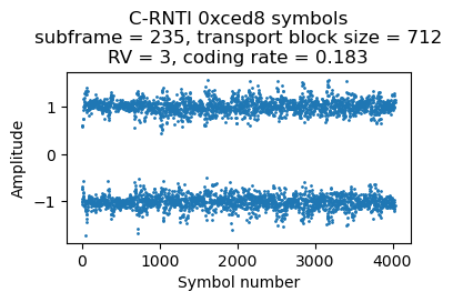
This situation happens again in subframe 235. There is the following DCI in subframe 221.
In subframe 235 (also 14 ms later), we find this DCI, which indicates that the first codeword is retransmitted. The set of RBs allocated to this retransmission is much smaller than the original set, because the original transmission had a much longer transport block in the second codeword. Now precoding matrix number 1 is used instead of matrix number 3.
Here are the symbols for this retransmission. The MAC PDU contains an 85 byte SDU.
Looking only at the coding rates of the retransmissions, we find that they are around 0.19. Thus, probably this UE is reporting CQI 3 (or CQI 2, if it supports 256QAM). It would be interesting to also look at the coding rates of the original two-codeword transmissions.
C-RNTI 0xc3c7
There are 3 PDSCH transmissions for C-RNTI 0xc3c7 in the first 500 ms of the recording. They are always rather short, with a transport block size of 56 bits and using resource blocks 36-38 (3 RBs), which gives a coding rate of 0.09 or 0.10 depending on the CFI. The symbols for the three transmissions are shown here.
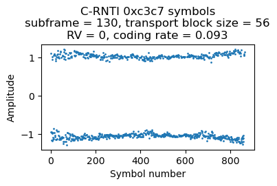
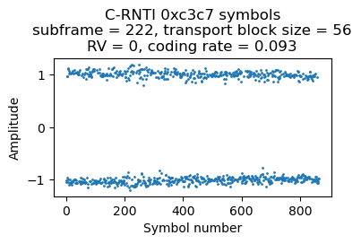
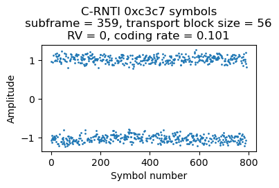
As we will see below, the first and third transmission are ACKs from the RLC layer AM mode (acknowledged mode). Looking at the PDCCH we see that there are many DCI format 0 messages for this UE containing uplink grants, so it looks like this UE is just uplinking data during this part of the recording.
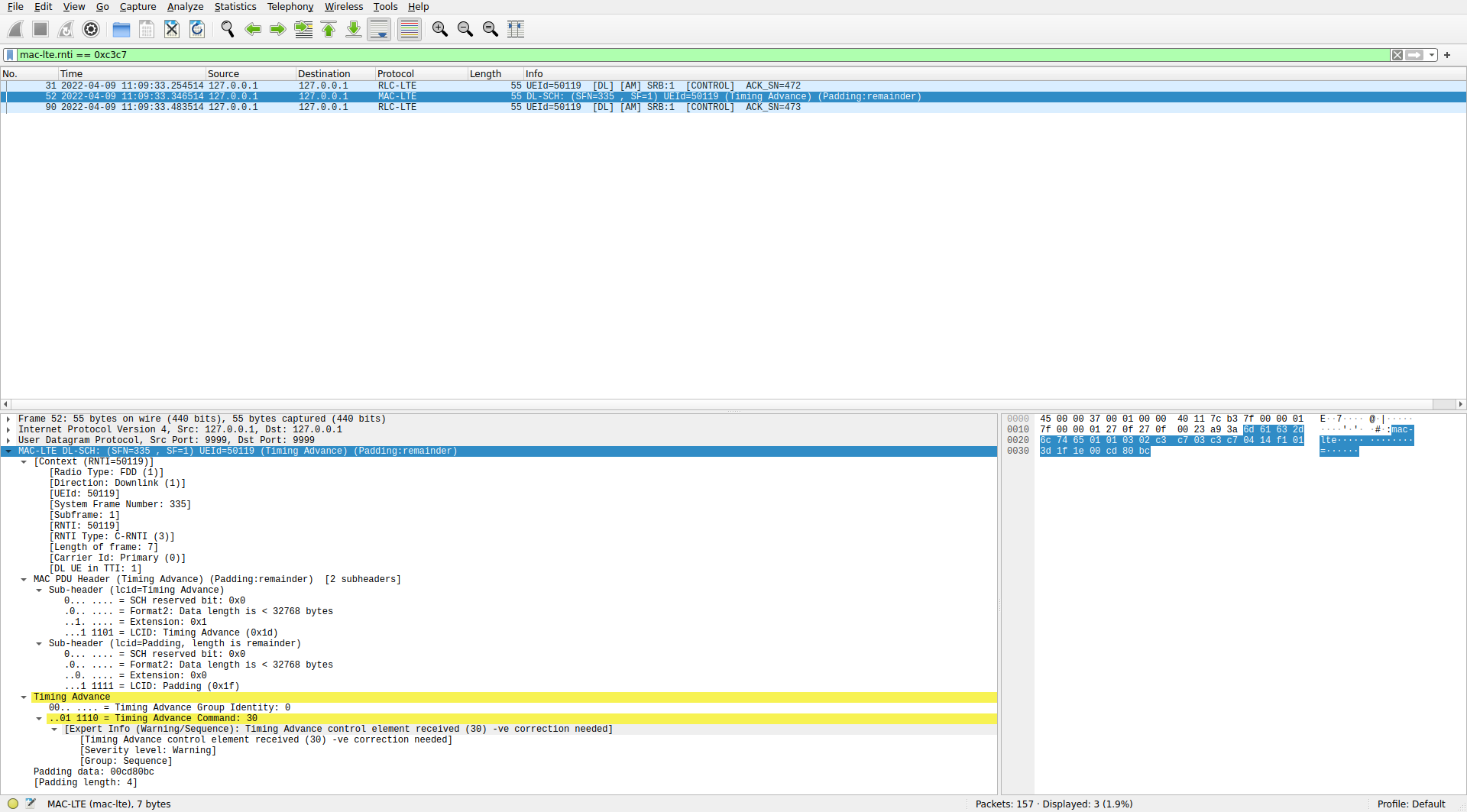
The second transmission is a timing advance command. The raw value of the command is 30. Using the formula to convert to units of time, this corresponds to a negative update of of -16 samples at 30.72 Msps (approximately -521 ns) with respect to the timing advance previously used by the UE. The timing advance has a granularity of 16 samples, so this command is the smallest timing advance tweak that can happen.
C-RNTI 0xcee3
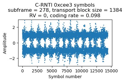
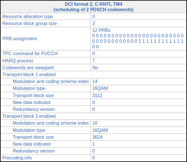
This is the most interesting UE in the recording because it is reporting a high CQI, so some of its PDSCH transmissions use 16QAM or 64QAM. The first transmission for this UE occurs in subframe 278. This is its corresponding DCI. The transport block size is relatively large, so all the 50 RBs of the cell are used. This gives a coding rate of 0.098.
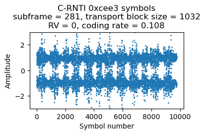
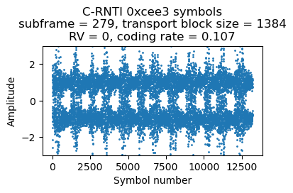
The second transmission comes in subframe 279. Its DCI looks almost identical, except the HARQ process is 6 because HARQ process 7 is still waiting for the ACK/NACK from the transmission in subframe 278. There is nothing for this UE in subframe 280. In subframe 281 there is the following DCI. The transport block size is smaller, so only 38 RBs are used (the coding rate is still around 0.1). This transmission needs to use HARQ process 5.
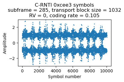
The next DCI for this UE comes in subframe 285. It is identical to the previous one except that HARQ process 4 is used.
Here are the plots of the symbols of each of these 4 PDSCH transmissions. The banding in the plots is caused by the fact that the transmissions use the whole cell bandwidth and in the recording there is less SNR in the lower part of the cell. Since the coding rate is around 0.1, the CQI is probably 1 or 2.
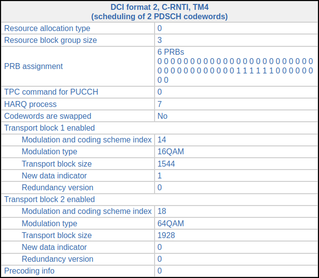
The next DCI for C-RNTI 0xcee3 appears in subframe 288. This now transmits two-codewords modulated with 16QAM. The coding rate is 0.5 and 0.58 for the first and second codewords respectively. It looks like the UE is now reporting CQI 8 (assuming that it doesn’t support 256 QAM; otherwise the CQI would be 5).
There is a very similar transmission in subframe 292. The only difference in the DCI is that it uses HARQ process 6. The next trasmission is in subframe 295. The modulation has been upgraded to 64QAM. The coding rate for the two codewords is 0.46 and 0.55, so it looks like the UE is reporting CQI 10 for the weaker MIMO channel mode (which carrier the first codeword) and CQI 11 for the stronger (which carries the second).

There are several more PDSCH transmissions in the next subframes, using a combination of 16QAM and 64QAM, and relatively large transport block sizes. All of them are two-codeword TM4, so we cannot decode any of them. Some transmissions use 16QAM for the first codeword and 64QAM for the second one.
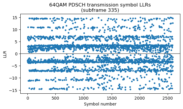
Our chance to decode something comes in subframe 335, where the DCI looks as follows. This is a retransmission of a codeword whose decoding by the UE has failed.
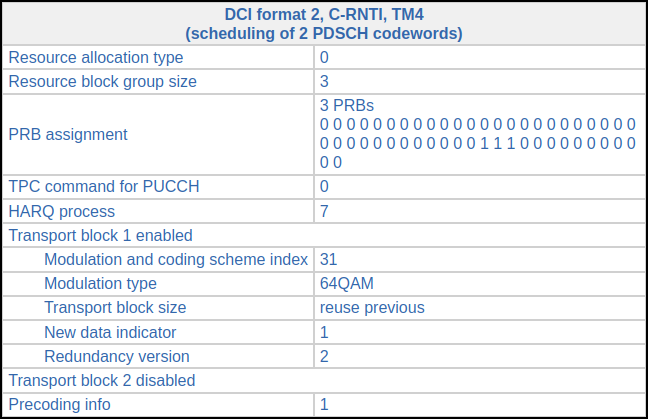
We need to go back and find the previous DCI for HARQ process 7 to find the transport block size. This happens in subframe 327 (exactly 8 ms before) and has the following DCI.
The original transmission for the first codeword uses 16QAM and a coding rate of 0.45 (CQI 8), while the second codeword uses 64QAM and a coding rate of 0.38 (maybe CQI 10). The retransmission of the first codeword changes to 64QAM and a coding rate of 0.6 (CQI 11 or 12).
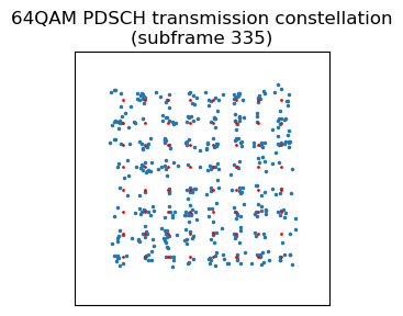
In order to decode this 64QAM retransmission, we first perform single-codeword TM4 equalization with the appropriate precoding matrix and plot the constellation diagram to check that the signal quality is good enough. The constellation of all the PDSCH resource elements in the transmission is shown in blue, and the reference constellation in red. The SNR and equalization is quite acceptable.
The next step is to obtain LLRs for each of the bits. We do this using the max*-safe function as in the post about TM4. In 64QAM, different bits in different symbols have different degrees of “protection” depending on how close they are to symbols encoding the opposite bit. This causes the horizontal bands in this plot of the LLRs. The LLRs make even more clear that the constellation plot the fact that the SNR is quite good and there are not many chances for bit errors (only for some parts of the “inner bands”).
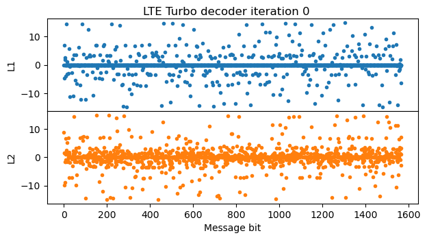
Now we need to descramble these LLRs. This is done in the same way as for LLRs or soft symbols coming from a QPSK transmission. Then we can run the Turbo decoder. It is very interesting to see how the message LLRs evolve on each iteration for this particular codeword. It almost looks like magic.
In the first iteration, many LLRs are zero after the pass of the first BCJR decoder. This transmission has a relatively high coding rate and a uses redundancy version 2, so the systematic bits are not transmitted. Therefore, the BCJR decoder doesn’t have enough information about most of the systematic bits. Things don’t look too good for the output of the second BCJR decoder either.
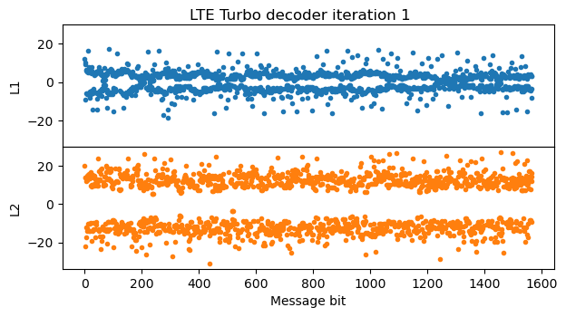
In the second iteration, after the first decoder has run, most parts of the message are well separated from zero and could be sliced without bit errors, but there are parts of the message where there are still bit errors. The second BCJR decoder fixes these parts. Decoding could really stop at this point, since now the message has no bit errors.
In the next iterations, the LLRs keep increasing. We also see that the effect caused by the lack of extrinsic information for the trellis termination starts to appear at the end of the message.
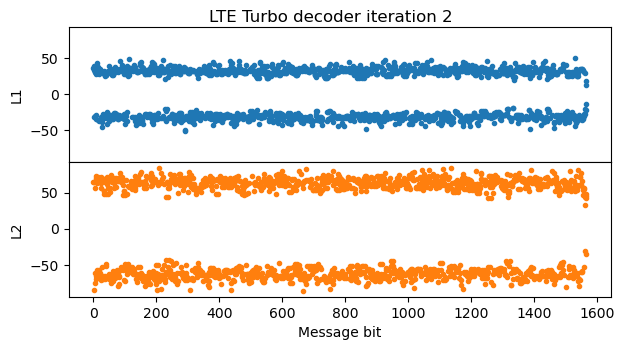
The LLRs keep increasing steadily with each iteration, until reaching around +/- 200 in the fifth iteration.
After the fifth iteration there is not much change in the LLRs, since they have almost converged. This is the final iteration of the algorithm.
Exporting decoded transport blocks to Wireshark
To analyze the contents of all the transport blocks we have decoded, Wireshark can be a very useful tool, since it can dissect several LTE layers and protocols: the MAC layer, the RLC layer, the PDCP protocol, and the RRC layer. There are several ways to format the transport blocks so that Wireshark can read them as LTE MAC layer frames. Probably the most straightforward is as the payload of UDP packets, using the format defined in packet-mac-lte.h. There is an example application mac_lte_logger.c that shows how to do this. Basically, the payload of a UDP packet addressed to port 9999 is filled with a fixed header, and then some optional headers and the transport block data. The presence of the optional headers and transport block data is indicated using tags. In Wireshark it is necessary to enable the mac_lte_udp protocol in the Analyze > Enabled Protocols… menu in order to dissect these UDP packets as LTE MAC frames.
These UDP packets can be sent over the network, but for analysis it is better to store them in a PCAP file (by putting each UDP packet into an IPv4 packet, for example). I’m using Scapy to generate the IPv4 and UDP headers, and to write the PCAP file. My code fills in some metadata in the packets, such as the SFN and subframe, and the RNTI. There is also a UE ID field in the Wireshark LTE MAC metadata. I’m filling this with the C-RNTI for C-RNTI frames, since I don’t have any other ID for the UEs. Additionally, I’m timestamping the packets in the PCAP using the timestamp that corresponds to the beginning of the subframe in which each packet was transmitted. These timestamps are generated using the receiver clock (count of IQ samples in the recording), so it is interesting to see how they drift slightly compared to the nominal rate of one subframe per millisecond.
Packet analysis in Wireshark
In this section I look at the PCAP file with Wireshark. You can grab the file and follow along (some settings that will be explained below are required). I don’t have a very good knowledge of the upper layers of LTE, so there might be some small mistakes or omissions in this analysis.
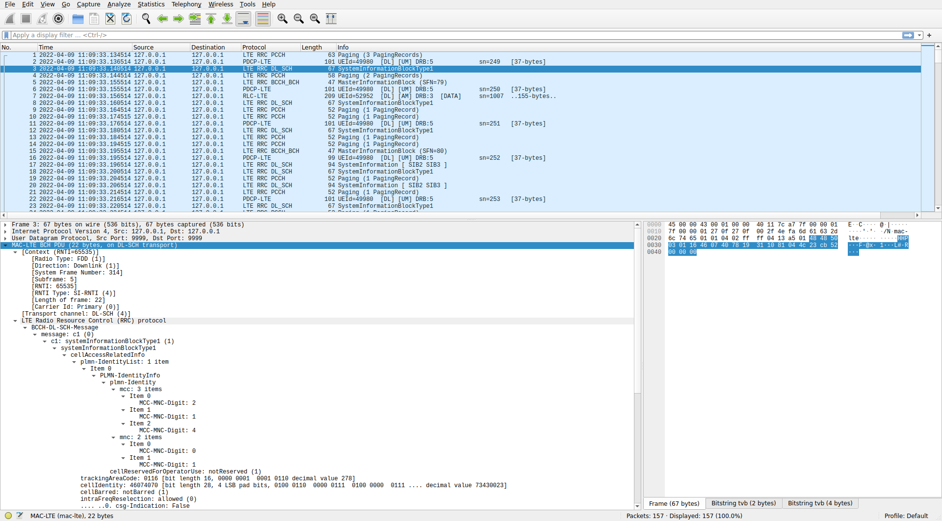
Here is how the PCAP file loaded in Wireshark looks like (click on the image to view it in full size).

The SIBs, the MIB and the paging messages are parsed using the RRC ASN.1, so we don’t see any new information, although Wireshark is quite convenient to inspect the values.
MAC PDUs from C-RNTIs are more interesting, since I haven’t been parsing those in the Jupyter notebook. Here is the first example of a MAC PDU in the PCAP file.
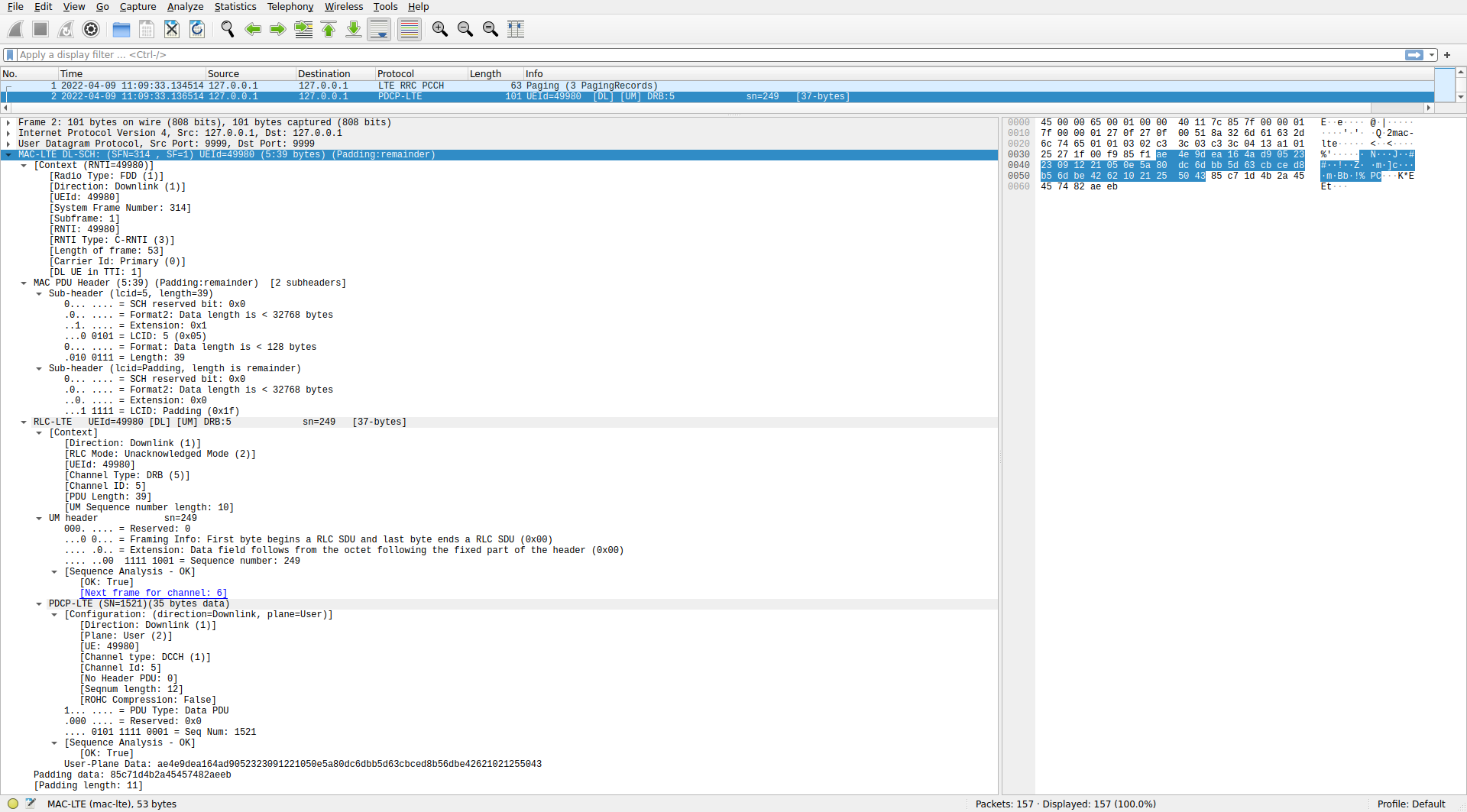
Under the MAC-LTE DL-SCH header we can first see the context, which is populated with metadata and calculated data (such as the number of DL UEs in this TTI). Then the MAC PDU header is parsed. A MAC PDU can contain several elements, which can be SDUs from the upper layer, control information (called control elements), or padding. Each of these elements is described with a sub-header. This is illustrated by the following figure. All the MAC PDUs I’ve decoded are relatively simple. They only have one item (SDU or control element) and padding.
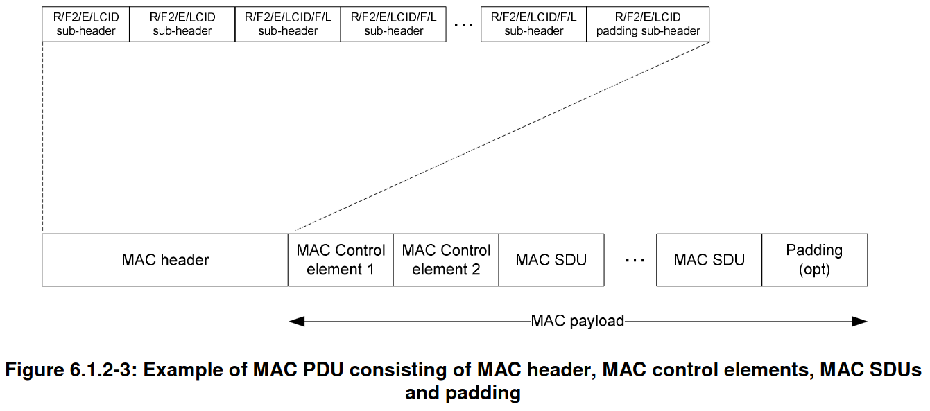
Padding is used to pad the MAC PDU to the transport block size that is selected for transmission. The transport block size is indicated indirectly through information in the DCI. The MCS determines the constellation and an index \(I_{\mathrm{TBS}}\). This index together with the number of allocated resource blocks \(N_{\mathrm{PRB}}\) determines the transport block size according to a table. Part of that table is shown here.
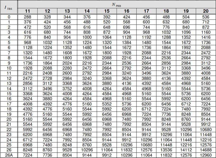
In the case of this MAC PDU, it uses 12 resource blocks and has a transport block size of 424 bits, so \(I_{TBS} = 1\). This is the value that corresponds to MCS 1. If we look at the MAC PDU in Wireshark, we see that it has 11 bytes (88 bits) of padding. I don’t know why this amount of padding was chosen by the eNB. The useful data is only 336 bits long. Looking at the table above, we see that the eNB could have reduced the amount of padding and allocated this transmission to 11 RBs, which has a transport block size of 376 bits with MCS 1, or even 10 RBs (not shown in the table excerpt), which has a transport block size of 344 bits. I haven’t found the reason why a smaller amount of padding, and hence less radio resources, is not used.
The first MAC sub-header in this PDU indicates the length of the data (39 bytes in this case) and contains an LCID (logical channel ID). The LCID identifies the kind of data that is contained in the element of the PDU described by this sub-header. LCIDs between 0 and 10 identify an SDU with upper layer data, while LCIDs above 16 identify control information (called MAC PDU control elements) and padding.
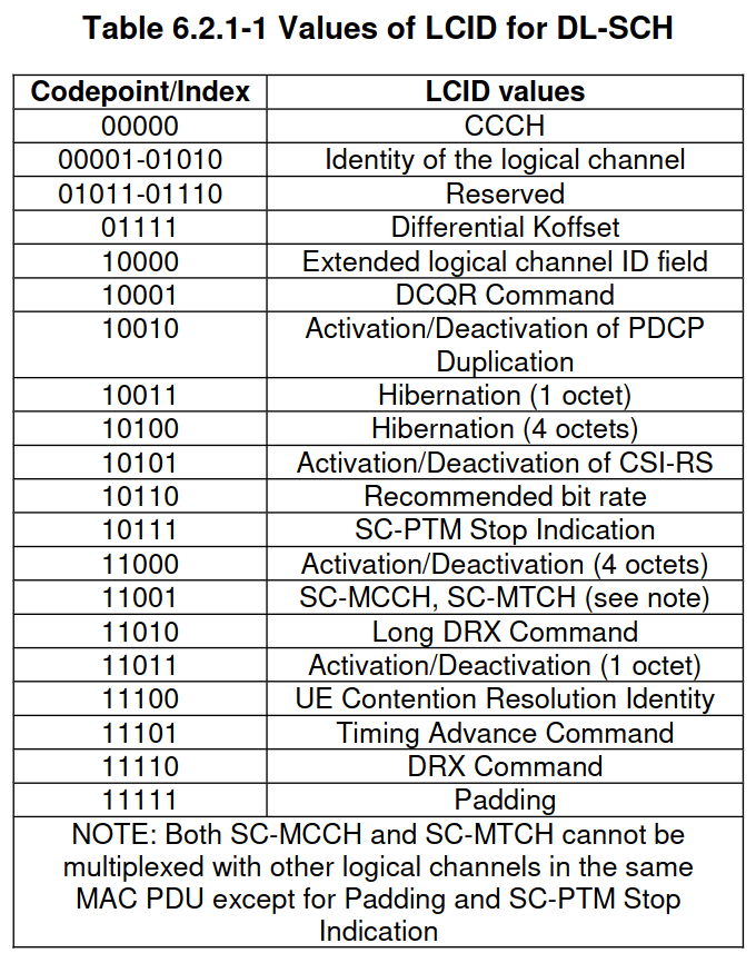
In this MAC PDU, the LCID of the first sub-header is 5, indicating that it refers to an SDU from logical channel 5. The second sub-header refers to the padding after this SDU, and uses LCID 0x1f to indicate that it is padding.
Here comes the tricky part. In order to parse the SDU, we need to know what kind of RLC protocol is used in logical channel 5. Usually, this would be communicated to the UEs by means of control information, but we haven’t seen that control information in the PDSCH transmissions that we have decoded. Wireshark has options to declare manually what protocol is used in each logical channel. These are in the MAC LTE protocol options, accessible either through “Edit > Preferences > Protocols > MAC-LTE”, or by right clicking on the packet in the packet list or on one of the MAC-LTE fields in the dissection of the packet and going to “Protocol preferences”.
The first of such options is “Attempt to dissect LCID 1&2 as SRB 1&2”. SRB stands for signalling radio bearer. A kind of control channel. I don’t know all the details, but this correspondence between LCIDs and SRBs seems to be popular enough that Wireshark offers an option for it. This option seems to work well for the MAC PDUs in this recording that use LCID 1, as we will see.
For LCIDs between 3 and 10 things are more difficult. These are to be mapped to DRBs (data radio bearer) through the setting “Source of LCID -> drb channel settings”. There is an option “From configuration protocols” to learn the mappings from control information. We cannot use this because we haven’t decoded this control information. The other option is “From static table”, which allows us to declare the mappings manually with the “LCID to DRBs mapping table”. In this table we need to enter the LCID, the DRB ID, and the RLC protocol used. With some messing around, I have arrived to the following settings.
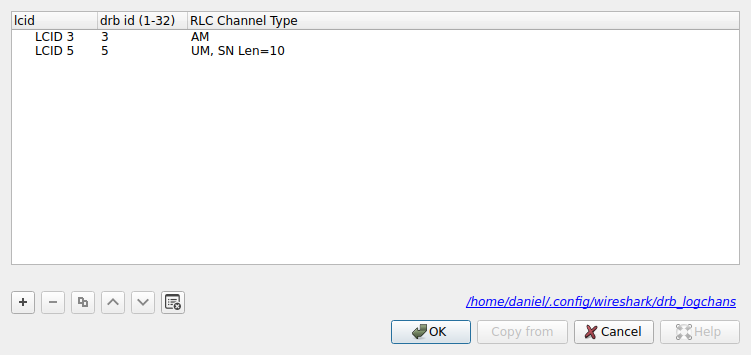
LCIDs 3 and 5 are the only ones that appear in the decoded MAC PDUs (besides LCID 1 and control elements). The DRB ID is not too important, so I’ve kept it the same as the LCID for simplicity. The key value is the RLC channel type, as Wireshark will use this to select how to dissect the SDU.
I am quite sure about assigning “UM, SN Len=10” to LCID 5, because this gives decodes that make sense for this LCID, and other assignments don’t. I am not so sure about the “AM” assignment to LCID 3. This is the best I’ve been able to find, but the results don’t look too convincing as we will see.
UM stands for unacknowledged mode. This mode adds segmentation (fragmentation) and concatennation to RLC SDUs, but this is the only extra functionality offered compared TM (transparent mode), which sends the RLC SDUs without any modifications. The UM header contains a sequence number and framing information, which indicates if the UM payload begins and/or ends an RLC SDU.
In this recording, LCID 5 is used only by C-RNTI 0xc33c. Above we saw that a PDSCH transmission is sent to this UE approximately every 20 ms. Below we see a Wireshark view of all the MAC PDUs for this C-RNTI. They all use LCID 5 and contain a 37 byte UM RLC PDU. The sequence numbers in the UM header are consecutive, which makes me confident that I’ve configured the RLC protocol for this LCID correctly.
0xc33c in WiresharkWe also see that Wireshark dissects the SDU carried by the UM PDU as a PDCP PDU. The PDCP protocol is what is used in LTE to carry user data, such as IP packets, as well as RRC (radio resource control) packets. The header in these particular PDCP PDUs has a sequence number and not much else. We can configure the PDCP protocol preferences in Wireshark by using the “Which layer to show in Info column > PDCP Info” to show the PDCP sequence number in the packet list instead of the UM information. In this way we can see that the PDCP PDUs have consecutive sequence numbers. Another confirmation that this data is being parsed correctly.
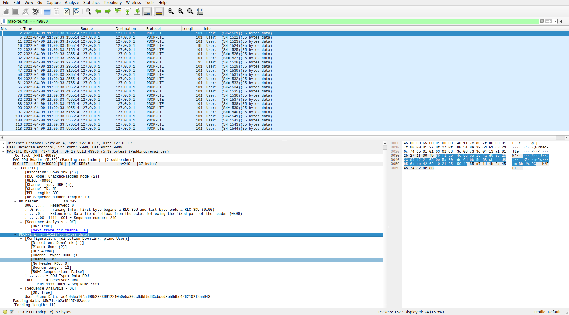
0xc33c in WiresharkThus we see that C-RNTI 0xc33c is receiving PCDP PDUs with 35 bytes of data through the RLC UM protocol on LCID 5 approximately every 20 ms. The PDCP payload is usually encrypted, and this seems to be the case here. Wireshark allows us to perform decryption if we supply the keys, but of course we don’t have them.
Now let’s look at the MAC PDUs for C-RNTI 0xc3c7. I already mentioned what these contain when I showed the PDSCH transmissions for this UE.
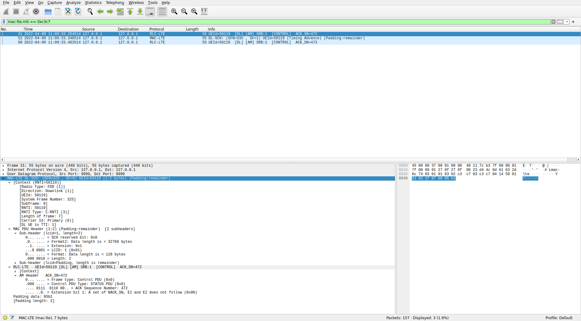
0xc3c7 in WiresharkThe first and third MAC PDUs contain an SDU from LCID 1. Wireshark dissects this as an AM RLC PDU from SRB 1, since we have the option “Attempt to dissect LCID 1&2 as SRB 1&2” enabled. AM stands for acknowledged mode, and it is an RLC protocol that provides delivery confirmation via ACK messages, in addition to the segmentation and concatenation capabilities provided by UM. The AM headers of these PDUs corresponds to an ACK control message. The ACK sequence numbers are consecutive. Therefore these seem good dissections of these messages.
The dissection of the second MAC PDU is shown below. This contains a single control element with a timing advance command. As mentioned previously, the value of the timing advance is 30, which corresponds to a timing advance update of -16 samples.
0xc3c7Now we come to the part where I’m not so certain that I’m dissecting the MAC PDUs correctly in Wireshark. Let’s first look at C-RNTI 0xced8. As mentioned above, this is a UE that is using two-codeword TM4, so we can only decode a PDSCH transmission when it is a retransmission of a single codeword. This happens only twice in the first 500 ms of the recording. The next figure shows these two MAC PDUs in Wireshark.
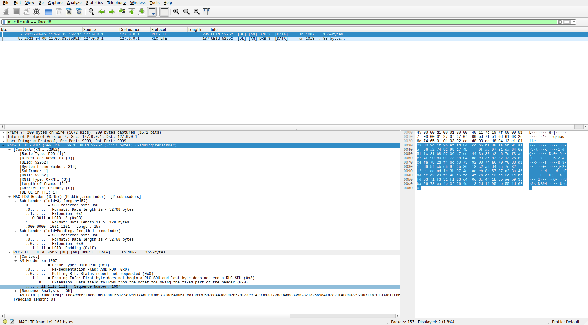
0xced8 in WiresharkBoth MAC PDUs have the same format. They carry an SDU with LCID 3. I have instructed Wireshark to dissect LCID 3 as AM. The dissection of the AM RLC PDUs shows that both PDUs contain a segment of the middle of an SDU (an RLC SDU doesn’t start nor end in this PDU). The sequence numbers are 1007 and 1013. These are close by, so at first glance it looks reasonable, since we’re failing to decode some MAC PDUs addressed to this UE. However, a closer look at the PDCCH decodes, shows that the following are the only PDSCH transmissions for C-RNTI 0xced8 in the first 500 ms of the recording:
Subframe index 18: CFI 1, CCEs 0-7, 59 bit DCI
CRC-16 mask 0xced8
DCI (hex, without CRC) 7c07ce101000

Subframe index 32: CFI 1, CCEs 0-7, 59 bit DCI
CRC-16 mask 0xced8
DCI (hex, without CRC) 7007ceeb0160

Subframe index 221: CFI 1, CCEs 0-7, 59 bit DCI
CRC-16 mask 0xced8
DCI (hex, without CRC) 7807ce041c20

Subframe index 235: CFI 1, CCEs 0-7, 59 bit DCI
CRC-16 mask 0xced8
DCI (hex, without CRC) 4003ceef0520
The transmissions that we’ve decoded are those in subframe 32 and subframe 235. They are retransmissions of the first codeword of the two-codeword transmissions in subframes 18 and 221 respectively. So between these two MAC PDUs we have only missed one MAC PDU: the second codeword of the subframe 18 transmission. Therefore, I don’t see how the AM sequence number could be jumping from 1007 to 1013.
Since the two AM PDUs contain a fragment of an RLC SDU (potentially a PDCP PDU), we can’t dissect this SDU, as we’re missing most of its data.
Let’s now look at the MAC PDUs for C-RNTI 0xcee3. All the five PDUs that I’ve decoded are shown here. As in the case of C-RNTI 0xced8, they also contain a single SDU with LCID 3, which is being dissected as AM.
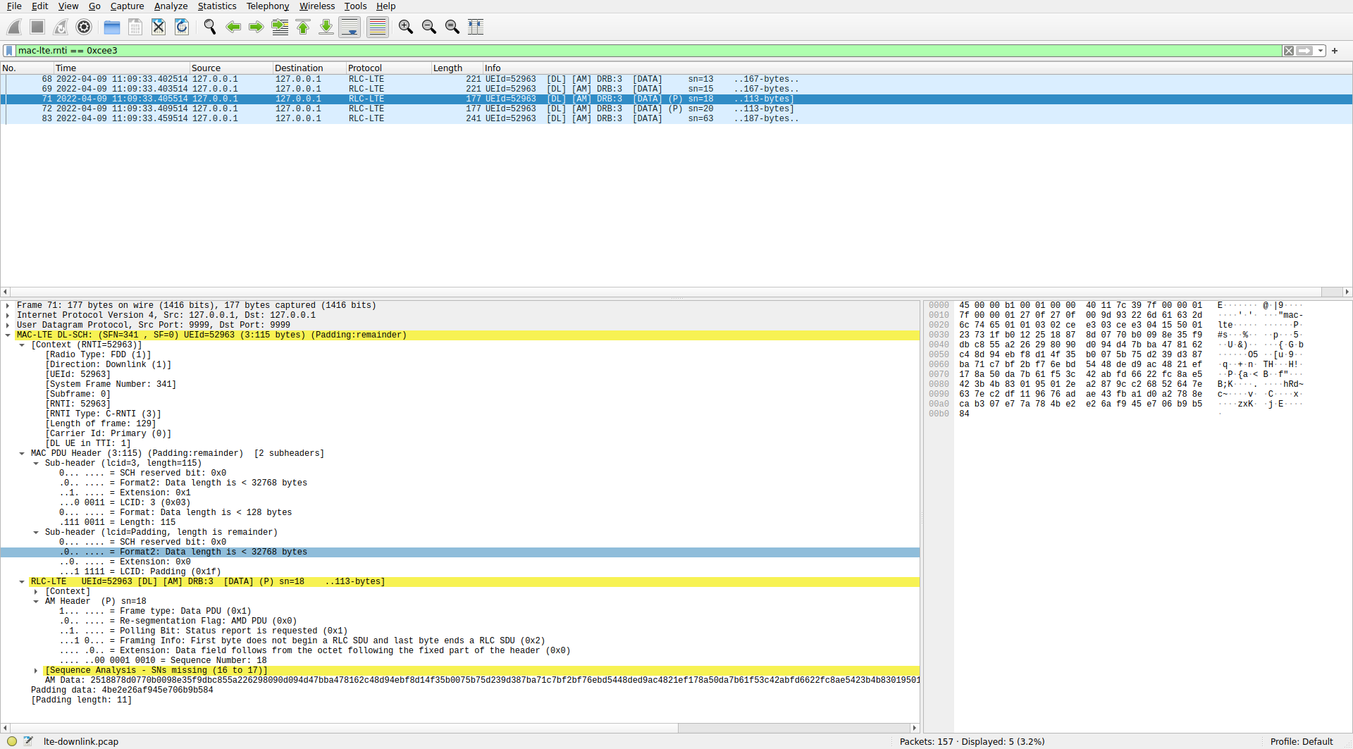
0xcee3 in WiresharkSome of the AM PDUs look like those of C-RNTI 0xced8, but there are also two PDUs in which an RLC SDU ends. These two PDUs also have the polling bit (P) set. The details of one of them are shown above.
As in the case of the AM PDUs of C-RNTI 0xced8, the sequence numbers are not consecutive. The first two MAC PDUs in this list were decoded from single-codeword TM4 transmissions in consecutive subframes (subframes 278 and 279). These were the two transmissions that occupied the whole 50 RBs of the cell and used low coding rate QPSK. So there can’t possibly have been any other PDSCH transmission between them. The third MAC PDU is from subframe 281, still a low coding rate single-codeword TM4 QPSK transmission (although this didn’t occupy the whole 50 RBs). There were no PDSCH transmissions for C-RNTI 0xcee3 in subframe 280. The fourth MAC PDU comes from subframe 285. It is a transmission with the same characteristics as the previous one, and there are no transmissions for C-RNTI 0xcee3 in subframes 282-284. Therefore, the first 4 MAC PDUs are consecutive, but for some reason the AM sequence numbers are 13, 15, 18, 20.
The final PDU is from the 64QAM transmission in subframe 335. The AM sequence number jumps from 20 to 63. As indicated above, subframe 335 was a retransmission of the first codeword of subframe 327. There were 10 PDSCH tranmissions for C-RNTI 0xcee3 between subframe 285 and subframe 327. All of them were two-codeword TM4, and I think none of them were a retransmission. Thus, this accounts for 20 MAC PDUs, which doesn’t explain how the AM sequence number can jump by 43.
Dissecting LCID 3 as AM doesn’t look wrong, in the sense that it doesn’t give anything that is clearly malformed. However the fact that the sequence numbers increase more than they should (but not by a huge amount) puzzles me. I don’t have a good explanation for what’s happening. Perhaps these UEs are receiving data from multiple cells (multiple bands perhaps), and so we only see part of the traffic.
Data and code
The Jupyter notebook where all the analysis in this post has done can be found here. This uses a SigMF recording that is hosted here. The RRC ASN.1 and the PCAP file containing the decoded transmissions is in the same repository.
2 comments