I am interested in monitoring the usage of the QO-100 WB transponder over several weeks or months, to obtain statistics about how full the transponder is, what bandwidths are used, which channels are occupied more often, etc., as well as statistics about the power of the signals and the DVB-S2 beacon. For this, we need to compute and record to disk waterfall data for later analysis. Maia SDR is ideal for this task, because it is easy to write a Python script that configures the spectrometer to a low rate, connects to the WebSocket to fetch spectrometer data, performs some integrations to lower the rate even more, and records data to disk.
For this project I’ve settled on using a sample rate of 20 Msps, which covers the whole transponder plus a few MHz of receiver noise floor on each side (this will be used to calibrate the receiver gain) and gives a frequency resolution of 4.9 kHz with Maia SDR’s 4096-point FFT. At this sample rate, I can set the Maia SDR spectrometer to 5 Hz and then perform 50 integrations in the Python script to obtain one spectrum average every 10 seconds.
Part of the interest of setting up this project is that the Python script can serve as an example of how to interface Maia SDR with other applications and scripts. In this post I will show how the system works and an initial evaluation of the data that I have recorder over a week. More detailed analysis of the data will come in future posts.
The Python script I’m using can be found here. It uses the Python requests package to configure Maia SDR using its REST API, the websockets package to connect to the spectrometer WebSocket, and NumPy to average groups of 50 spectra together and write them to a file, as well as writing timestamps to another file. Dealing with the spectrometer WebSocket is really simple. Each message provides a 4096-point spectrum (in linear unit), which we can convert to a NumPy array by doing
np.frombuffer(await ws.recv(), 'float32')The script produces two output files: a file with the spectrum data in float32 format, and a file with the timestamps in datetime64[ns] format.
I have set up a Pluto in my shack connected to the 750 MHz IF of my QO-100 groundstation. A LimeNET board that I had around is acting as USB to Ethernet bridge, but any Raspberry Pi or similar board, or a USB Ethernet adapter could also be used. In this way, I have network access to the Pluto from my home network. The Python script is run in a server at home (again, a Raspberry Pi or any other board with enough storage could be used, since the script doesn’t require much CPU). A gain of 50 dB works well for the signal levels that I have in this set up, but this can be changed with one of the script command line parameters. I started recording data last Sunday, so I already have one week worth of data.
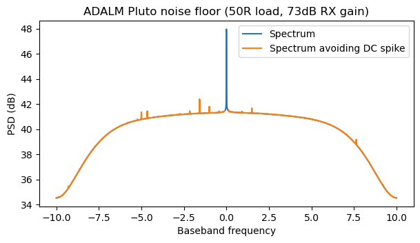
To obtain more accurate results when measuring signal power, I have calibrated the bandpass of the Pluto. To do this, I connected a 50Ω load to the RX port of the Pluto and used the same script to record some data. I increased the RX gain to the maximum, which is 73 dB, because with a gain of 50 dB the shape of the noise floor is totally different from the one we see when there is enough noise at the input. The rest of the settings are the same ones that I’m using to record the WB transponder. I’ve used a different Pluto to do this calibration, since I had already started the recording of the WB transponder and didn’t want to stop it. I guess that this doesn’t make much difference. I’m mainly interested in calibrating out the shape of the passband caused by the decimating filters of the AD9363, and these digital filters are the same for all Plutos. I have recorded 720 seconds of data, but it isn’t necessary to record for so long.
The following figure shows the spectrum averaged over all the data. There are a few weak spurs, as well as the DC spike. I’m ignoring the DC spike in my fit, so I make a frequency selection that avoids it.
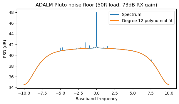
Next I perform a polynomial fit to the power spectral density (in linear units). I have found that using a polynomial of degree 12 gives a very good fit.
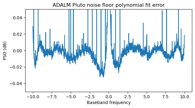
The next figure shows the error of the polynomial fit. It is on the order of 0.02 dB, which is very good. Also, the error is not symmetric, so at this point we are looking to effects different from the AD9363 digital filters (which have a symmetric response).
We can now use the polynomial obtained above to flatten out the bandpass response in our QO-100 WB transponder data. The next figure shows the first spectrum in the data I have recorded, with the bandpass calibration applied. I have marked in orange the parts of the spectrum that will be used to measure the receiver noise floor. This is the part of the spectrum that is away from the transponders (note that the signals from the NB transponder are also visible around 10490 MHz due to polarization leakage). I have also avoided a strong spur at 10503.02 MHz. The noise floor is not very flat. This may be due to the response of the LNB and the rest of the system, which we have not calibrated, or to differences between the two Plutos.
The receiver noise floor is used to estimate and calibrate the receiver gain. The gain of the amplifiers in the LNB depends on temperature and other factors, so it is important to calibrate the gain somehow if we want to make accurate power measurements. Note that this kind of calibration assumes that the receiver noise temperature is constant. This is not completely true, but it is probably the best we can do without injecting a reference signal of known power.
This figure shows the power of the receiver noise floor, measured by averaging the parts of the spectrum marked in orange above. We see how the noise floor goes up by about 0.8 dB at night, due to the lower temperatures increasing the gain of the LNA.
We divide the data by the receiver noise floor power, in order to calibrate out the receiver gain variations over time. The following shows the average spectrum over all the dataset, as well as a min hold and a max hold.
The min hold shows the shape of the transponder noise floor, which is slightly slanted. It also shows that the beacon dropped at some point by 4 dB. As we will see in future posts, this only happened briefly and seems to be an unusual situation. I find it interesting that in the average we can see the 5 rightmost channels of the transponder bandplan, since apparently people tend to use these channels more frequently, and often with 333 ksyms signals. The other channels do not show up well in the average due to a mixture of different signal bandwidths being used.
The max hold shows that sometimes there are very strong signals in the transponder. There seem to be moments in which the transponder is saturated and distortion products (shoulders) appear outside the typical ~9 MHz receive filter bandwidth.
Finally, here is a waterfall image that shows the signals during this week.
The code and Jupyter notebooks used in this post can be found in this repository. For the time being, I am not sharing the data because it amounts to 135 MiB per day, the files keep growing, and I don’t have a convenient way to share it. If someone is interested in getting access to this data, just let me know and I’ll figure out something.
2 comments