Since some years ago, a Doppler correction block has been available in gr-satellites. This block uses a text file that defines a time series of frequency versus time, and applies the appropriate frequency shift to each sample by linearly interpolating the frequency corresponding to the time of that particular sample. It can be used both to correct Doppler in a satellite propagation channel and other similar channels, as well as to simulate Doppler.
For some time I have been wanting to implement a similar block that applies a time-dependent delay to a complex baseband signal. The delay versus time would be defined by a text file in the same way as for the Doppler correction block. With this block, the delay of a satellite propagation channel can be simulated. It can also be used to correct the delay-rate of a satellite channel, which causes waveforms to be expanded or compressed in time due to a changing time-of-flight. This effect is known as code Doppler in GNSS, and as symbol frequency offset in general digital communications.
For accurate simulation of a satellite propagation channel, both the Doppler block and the delay block are needed, since the Doppler block accounts for the effects of variable time-of-flight on the RF carrier, and the delay block accounts for the effects on the band-limited modulation of the signal, by delaying its complex baseband representation.
I have now added a Time-dependent Delay block to gr-satellites. In this post I give a few details about its implementation and usage.
The Time-dependent Delay block uses a combination of GNU Radio’s history and a polyphase filterbank to apply a delay to a signal. The history is used to apply the integer part of the delay expressed in units of samples. By using history, the block can look back \(N\) samples in the past to produce its output. An advantage of having the delay file prepared ahead of time is that the block can determine the maximum delay that is needed when it is constructed, and call set_history() accordingly for this maximum history. When prototyping the implementation, I was somewhat concerned that I might hit some circular buffer size limits when requesting a large history. However, even requesting a few millions of samples of history doesn’t cause any errors.
A polyphase filterbank is used as a fractional delay filter. Each of the \(M\) arms of the filterbank implements a fractional time advance ranging from 0 to \((M-1)/M\) samples. This time advance is used to implement the fractional part of the delay in units of samples. To improve the quality of the filter, linear interpolation between two adjacent arms is used. In more detail, to apply a fractional time advance of \(0 \leq \tau < 1\) samples, the filter outputs corresponding to time advances \(\lfloor\tau M\rfloor/M\) and \((\lfloor\tau M\rfloor+1)/M\) are computed, and then the outputs are linearly interpolated with weights \(1 – (\tau M – \lfloor\tau M\rfloor)\) and \(\tau M – \lfloor\tau M\rfloor\) respectively. The relevant theory about this approach is in Section 7.5.2 of the book by fred harris.
This idea is very similar to how the Polyphase Arbitrary Resampler block works. I intended to reuse code from this block, but the code that manages the resampling ratio in that block is ingrained in the polyphase filterbank implementation. The Time-dependent Delay block is simpler, in the sense that the delay-rate is assumed to be small enough that it can act as a sync block, so it does not need to account for resampling. The philosophy of the operation of this block is that for each received (output) sample, the corresponding delay is computed, and then the transmit (input) sample corresponding to that delay is calculated by using the history to perform the integer part of the delay and applying the polyphase filterbank to perform the fractional part of the delay. That transmit sample is used as the output of the block. Therefore, the input-to-output sampling ratio relation of the block is always 1:1.
As usual, applying an FIR filter introduces an additional delay. In the case of the polyphase filterbank, the delay for the first arm is \(\tau_0 = (L-1)/(2M)\) samples, where \(L\) is the number of taps of the prototype filter. In general, arm \(j\) has a delay of \(\tau_j = \tau_0 – j/M\) samples. This FIR delay is taken into account by subtracting \(\tau_0\) from the delay that needs to be applied to the sample. For simplicity, it is required that all the delays in the text file are greater or equal than \(\tau_0\), so that the delay can be realized as the FIR delay plus an additional delay.
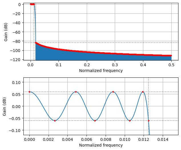
The prototype filter needs to be computed externally and supplied to the block as a vector of floats. In the example flowgraph for this block I am using pm-remez to design the filter. I have used the polyphase filterbank example in the pm-remez documentation to design a filter that is reasonably good for most use cases. The filterbank has 32 arms, which is a common choice, 18 taps per arm, and a transition bandwidth of 20%. With a stopband to passband weight ratio of 100 and \(1/f\) stopband response, this gives the following filter. Stopband rejection is better than 80 dB, while passband flatness is around 0.05 dB.
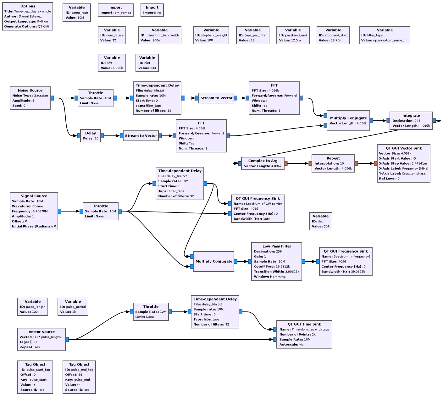
The example flowgraph looks like this. It has three distinct parts that are intended to show and test different effects caused by the time-dependent delay.
This flowgraph is to be used with a very simple delay text file. Each line of the text file contains the time in seconds (as in the Doppler correction block this can be time relative to the start of the simulation, absolute UNIX time, or any other kind of timestamp), and the delay in seconds. The example delay file looks like this:
0.0 1e-6
10.0 1e-6
20.0 2e-6
120.0 2002e-6
This means the following. For the first 10 seconds of simulation, the delay is fixed at 1 usec. Over the next 10 seconds the delay increases to 2 usec. For the next 100 seconds the delay increases by 2 ms, reaching 2002 usec. This corresponds to a delay-rate of 20 ppm, which is the typical order of magnitude of a LEO satellite channel (it corresponds to a range-rate of around 6 km/s).
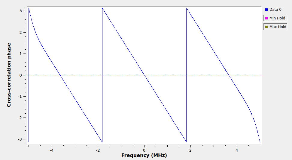
The first section generates AWGN, applies a time-dependent delay and a fixed delay of 10 samples (1 usec) to it, computes the cross-correlation, and plots the phase versus frequency of the cross-correlation. The relative delay between the Time-dependent Delay block output and the fixed 1 usec delay output can be read from the slope of the phase versus frequency of the cross-correlation. During the first 10 seconds of simulation, the Time-dependent Delay block is generating a delay of 1 usec, so the phase versus frequency plot is flat. Then it starts decreasing in slope as the time-dependent delay increases, as the following figure shows.
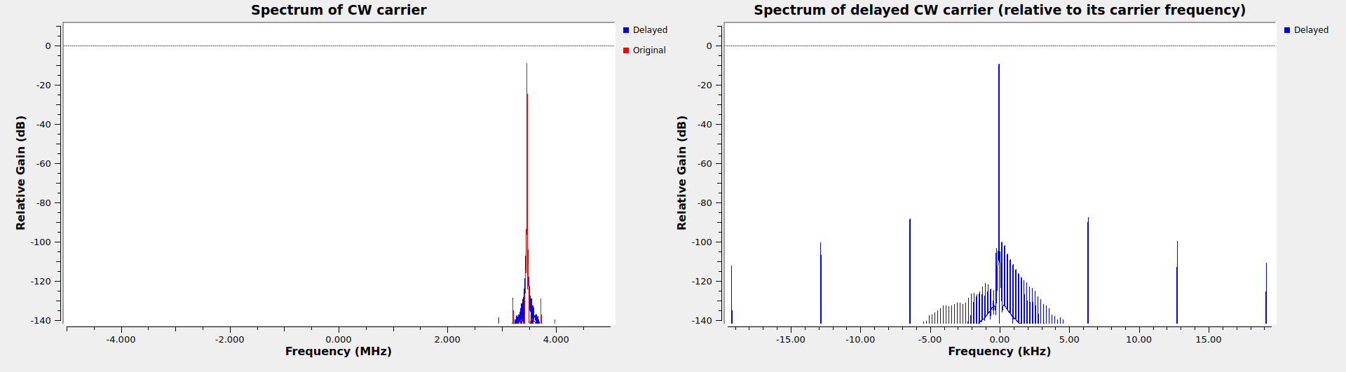
The second section generates a CW carrier at a frequency of about 3.45 MHz in complex baseband, and applies the Time-dependent Delay block to it. This section is used to evaluate the spurs produced by the fractional delay filter, as well as to look at the frequency shift produced by the delay-rate. Two plots are shown. The first shows the spectrum of the original and delayed CW carrier. The second one mixes the delayed carrier with the original carrier (as a simple way of removing the frequency offset corresponding to the original carrier), and decimates to show the behaviour close to the CW carrier. These plots are most interesting to look at during the part of the simulation when a delay-rate of 20 ppm is applied. In this case, the resampling spurs are at -78 dBc, and the delayed CW carrier shows a frequency shift of about -70 Hz (which is about right, since 3.45 MHz times 20 ppm gives 69 Hz).
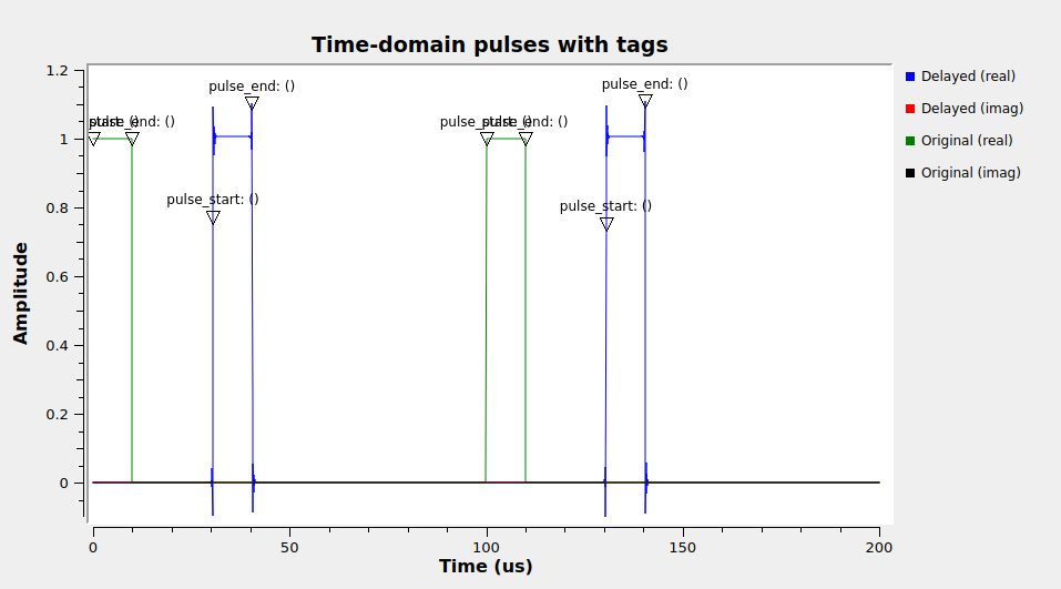
The third section is intended to test tag propagation. It generates periodic pulses with tags marking the first and last sample of each pulse. Pulses are run through the Time-dependent Delay block and compared in a Time Sink with the original pulses. The edges of the pulses are somewhat smeared by the fractional delay filter, but the tags always appear in one of the samples of the pulse edge.
Implementing tag propagation in this block is slightly tricky. The way I have done it is as follows. When a tag arrives to the input, the delay \(\tau(t_i)\) corresponding to the time \(t_i\) of that input sample is calculated. The tag offset is advanced by that delay rounded to an integer number of samples. Note that this is an approximation that assumes that the change in delay over a time period corresponding to the delay is very small (formally, \(|\tau'(t)\tau(t)| \ll 1\, \mathrm{sample}\)). The reason is that the proper way of propagating tags would be, for each time \(t_o\) corresponding to an output sample, find the delay \(\tau(t_o)\) and put into this sample any tags that were carried in the sample corresponding to time \(t_i = t_o – \tau(t_o)\). The approximation I am doing assumes \(\tau(t_o) \approx \tau(t_i)\). Since tags always need to be assigned to an integer offset, the delay \(\tau(t_i)\) is rounded to an integer number of samples.
Another detail regarding tag propagation is that rather than directly placing tags at offset \(t_i + \tau(t_i)\), they are temporarily stored in an internal vector until the work() call in which the block produces the sample corresponding to time \(t_i + \tau(t_i)\). This is not strictly needed, since a block can produce tags “in the future” that correspond to offsets to be be produced in future work() calls. However it might be a good idea to avoid putting too many tags into the output buffer which don’t need to be present yet.
The easiest way to use the Time-dependent Delay block is to copy the Variable cells used to design the FIR filter in the example flowgraph. This FIR filter should be appropriate for most use cases. The parameters in some Variables can easily be customized if some aspects of the filter needs to be modified for a particular application. This might be to achieve lower computational cost, lower spurs, or smaller transition bandwidth.
Besides the example flowgraph, I have also added an example Python script that generates a delay text file from a TLE and a groundstation location. This is similar to the Doppler correction Python script. The delay generation Python script can be used to create a delay file for delay simulation, and also for delay correction. In the case of delay correction, the sign of the delay needs to be inverted with the --invert-delay argument, and a constant positive delay needs to be added with the --delay-offset argument to make the resulting delay always larger than the minimum realizable delay given by the FIR filter delay.