I have been playing with some LTE recordings to brush up my knowledge, since it isn’t a protocol I’m very familiar with. I’m specially interested in understanding the structure and properties of all the pilot signals. Textbooks and documentation are great, but nothing beats getting your hands dirty with some IQ recordings to be sure you understand all the details.
To have something to work with, I have done some recordings of my phone by holding it near a USRP B205mini without an antenna. While recording, I was playing a Youtube video or browsing the web, to have some traffic. A waterfall of one of the recordings can be seen below. In this post we will be looking at how to demodulate the highlighted section, which contains 7 ms of PUSCH (physical uplink shared channel) occupying 15 resource blocks, together with the corresponding DMRS (demodulation reference signal) symbols. The post assumes some familiarity with OFDM, but doesn’t require any previous knowledge of LTE, so it can be useful to people interested in a hands-on introduction to LTE.
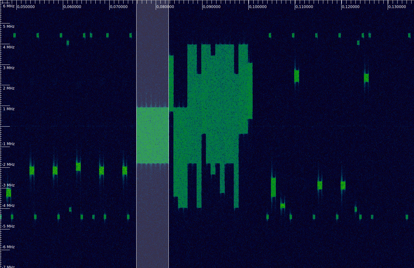
The recording can be found here. It is the SigMF file LTE_uplink_847MHz_2022-01-30_30720ksps. This contains 886 ms of data recorded at 30.72 Msps, and has much more than what we will be looking at here (in fact there is a PRACH right at the beginning). In this recording, my phone happens to be using Band 20. Specifically, a 10 MHz channel at 847 MHz. The demodulation is done in a Jupyter notebook using NumPy.
The documentation that describes how the LTE signals are modulated is 3GPP TS 36.211. I find this document a bit hard to read, because it often treats many special cases at once (which depend on a good number of parameters), and it isn’t obvious which is the case that is used most of the time. There are other online references that make a good job at summarizing the material, and have some very helpful diagrams. For instance, this one from Keysight. However, these are often not detailed enough, so a read through the 3GPP documents is needed.
LTE signal structure
Except in some special cases, the LTE signal is an OFDM modulation using a carrier spacing of 15 kHz. LTE is intended to work with a 30.72 Msps sampling clock for a 20 MHz bandwidth signal, so the timing parameters are defined in terms of samples at this clock rate. The useful time of a symbol is ~66.666 us (the reciprocal of 15 kHz), or 2048 samples (so that the OFDM DFTs can be implemented as an FFT of this size, which is a power of two).
The basic unit of duration is a slot, which lasts for 0.5 ms and consists of 7 OFDM symbols. The first symbol uses a cyclic prefix of 160 samples (~5.2 us), while the remaining symbols use a cyclic prefix of 144 samples (~4.7 us). We can check that the math adds up, because 7*2048 + 160 + 6*144 gives 15360 samples, which is exactly 0.5 ms. In time-frequency, allocations are done in terms of resource blocks, which have a time duration of one slot and a frequency span of 12 subcarriers.
The main channel in the uplink is the PUSCH (physical uplink shared channel), which is used to send data from the user equipment (phone) to the eNodeB (base station). In a slot of PUSCH, the first 3 symbols carry data using QPSK, 16QAM or 64QAM, the symbol in the middle is the DMRS (demodulation reference signal), which is a pilot signal for synchronization and equalization, and the last 3 symbols also carry data.
The data symbols of the PUSCH use SC-FDMA, while the DMRS uses regular OFDMA. The SC-FDMA modulation is often explained in terms of a precoder. If we have \(M\) continguous subcarriers allocated to our UE (user equipment), in OFDMA we would take \(M\) QPSK (or QAM) symbols and compute their inverse Fourier transform to obtain the corresponding time-domain OFDM symbol (taking into account that the OFDM subcarriers not allocated to our UE should be zero). This is often done by zero-padding the \(M\) symbols to obtain a vector of 2048 elements (zero-padding is done according to which \(M\) subcarriers are allocated), and then performing the 2048-point inverse DFT. In SC-FDMA, before doing this step, we use a precoder, which is simply an \(M\)-point DFT. This means that we compute the \(M\)-point DFT of our QPSK (or QAM) symbols, and then use that output to produce an OFDM symbol using an inverse Fourier transform in the same way as with OFDMA. The receiver will use an \(M\)-point inverse DFT to undo the action of the precoder.
An alternative way to explain SC-FDMA which I think makes more clear what is going on and why it is useful is the following. An SC-FDMA symbol consists essentially of \(M\) time-domain QPSK (or QAM) symbols being transmitted one after each other as a PAM waveform, at a rate of \(15 M\) kbaud. The pulse shape used for these symbols is such that they occupy the spectrum of the OFDMA subcarriers allocated to our UE, and, more importantly, such that these symbols are orthogonal to symbols transmitted by other UEs, which have other disjoint sets of OFDMA subcarriers allocated. As any OFDM symbol, an SC-FDMA symbol has a cyclic prefix, which can be used for channel equalization in the usual way. This cyclic prefix consists of the last few of our \(M\) QPSK (or QAM) time-domain symbols being sent before the first ones.
The advantage of SC-FDMA in comparison with OFDMA is that its PAPR (peak-to-average power ratio) is much smaller. The reason is that SC-FDMA is essentially a time-domain PAM waveform, so its PAPR is moderate. On the other hand, plain OFDM has huge peaks when many subcarriers happen to align in phase by chance. For this reason, SC-FDMA is used in the LTE uplink, since it is easier to amplify it efficiently, which is important for battery-powered UEs, as they have energy constraints.
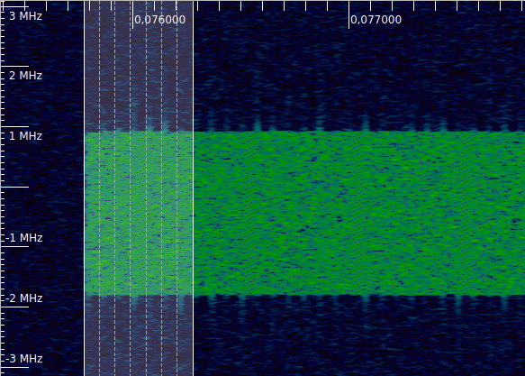
With the appropriate time-frequency resolution, it is possible to tell the SC-FDMA PUSCH symbols and the OFDMA DMRS symbols apart due to their different texture in the waterfall. The figure below shows an example of this, using cursors to delineate the 7 symbols in the first slot. The symbol in the middle is the DMRS, and it is possible to see that its texture is more regular, almost looking like a pattern. This contrast can also be seen in the next slots.
Coarse time synchronization: poor man’s Schmidl & Cox
Usually, the first step in demodulating OFDM is to achieve some coarse time synchronization with the symbols. Otherwise the FFTs we do might take up the last half of one symbol and the first half of the next symbol, and the result will be garbage.
Here I’m assuming that we already have coarse frequency synchronization, to within a fraction of the subcarrier spacing. If not, we will also need to find a way to estimate the carrier frequency offset. In our case this is not really needed, because at 847 MHz the frequency error will be a few kHz for devices having references accurate to a few ppm. The LTE subcarrier spacing of 15 kHz will typically be much larger than this.
However, we need to take into account that the subcarriers of the LTE uplink are laid so that there is no subcarrier at DC. The central subcarriers are at +7.5 kHz and at -7.5 kHz. More formally, the uplink subcarriers are at \((n+1/2)\Delta f\) for integer \(n\), where \(\Delta f = 15\) kHz is the subcarrier spacing. The usual demodulation of OFDM using an FFT has a subcarrier at DC, or in other terms, assumes that the subcarriers are at \(n \Delta f\) for integer \(n\). Therefore, to account for this difference we shift up our IQ recording by 7.5 kHz so that the subcarrier at -7.5 kHz is now placed at DC. Equivalently, we assume that our signal has a carrier frequency offset of -7.5 kHz to begin with.
Since we are analysing by hand a recording of the uplink, we need to do things somewhat differently from what an eNodeB receiving the uplink would do. In fact, UEs are responsible for their transmissions so that they arrive to the eNodeB at the correct moment, taking into account propagation delay. In this sense, the LTE uplink is synchronized in terms of the downlink. The eNodeB doesn’t need to perform coarse time synchronization. The symbols must already arrive synchronized to the eNodeB. Because of this, the LTE uplink doesn’t really have structures intended for coarse symbol synchronization, so we need to be a bit creative.
In this case coarse synchronization is easy, because we are attempting to synchronize to the beginning of a PUSCH transmission. There is no signal immediately before, so we could power-detect this beginning. An alternative idea is to use the fact that the DMRS symbols can be seen in the waterfall, so by looking at it we can have a rough idea of when the DMRS symbols start, which gives us the timing for all the other symbols. In fact, that is how I have aligned the markers in the figure above. This technique can be used even in the middle of a PUSCH transmission.
However, the technique I will use is what I call a poor-man’s Schmidl & Cox algorithm. The Schmidl & Cox algorithm requires specially crafted “preamble” OFDM symbols such that, in the time domain, the first half of the useful symbol is equal to the second half of the useful symbol. This property is achieved by only using even subcarriers, since all even subcarriers have this periodic property. When we have such a “preamble” symbol, we can compute the correlation\[C(t) = \int_0^{T_u/2} x(t + s) \overline{x(t + T_u/2 + s)}\,ds,\]where \(T_u\) denotes the useful symbol length and \(x(t)\) is the received waveform. This correlation will peak when \(t\) is equal to the start of the useful symbol of each of these “preamble” symbols. The way it works is by attempting to correlate the first half of a symbol with its second half, which gives a large value when these two halves are equal.
If our OFDM waveform doesn’t have these periodic “preamble” symbols, we can still use the same idea by relying on the cyclic prefix. This doesn’t work so well regarding sensitivity, because the cyclic prefix is usually much shorter than \(T_u/2)\), but can still be made to work with good SNR. The correlation we compute is\[\widetilde{C}(t) = \int_0^{T_{cp}} x(t+s)\overline{x(t+T_u+s)}\,ds,\]where \(T_{cp}\) denotes the length of the cyclic prefix. Since the cyclic prefix repeats exactly what happens at the end of the symbol, this correlation will peak when \(t\) is equal to the start of the cyclic prefix of each symbol.
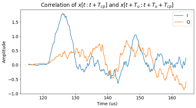
The result of applying this technique to our PUSCH transmission can be seen below. The waveform \(x(t)\) starts somewhat before the first PUSCH symbol, so that we don’t miss its beginning.
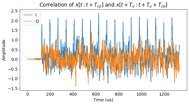
We can actually see three different amplitude levels in the figure. At the beginning the amplitude is very small, because both \(x(t)\) and \(x(t+T_u)\) are before the start of the PUSCH transmission, so they only contain noise of small amplitude. Then we can see a small increase in amplitude, which happens when \(x(t+T_u)\) reaches the first symbol but \(x(t)\) is still small amplitude noise. Finally, \(x(t)\) reaches the first symbol and we can see the peak produced by the cyclic prefix. The amplitude of the correlation is now larger even when there is no peak, since both \(x(t)\) and \(x(t+T_u)\) contain pieces of the OFDM signal.
The peaks we see in the figure correspond to the start of each cyclic prefix, so we can use them to count symbols. With some effort we could even be able to tell that the first out of every 7 symbols is slightly longer (due to its slightly longer cyclic prefix).
The figure above has been obtained with no carrier frequency error, so in some sense we’re still using the textbook’s trick of “assume that the signal is synchronized”. What happens when we have some carrier frequency error? If we replace \(x(t)\) by \(e^{2\pi i f t}x(t)\), we see that \(\widetilde{C}(t)\) simply gets multiplied by a factor \(e^{-2\pi i f T_u}\). Thus, we still get correlation peaks of the same amplitude, but they are no longer real and positive. Their phase indicates the frequency error (modulo the carrier frequency separation \(1/T_u\)), so as a bonus, this poor man’s Schmidl & Cox can also be used to achieve a rather precise frequency synchronization (the same is true of the usual Schmidl & Cox algorithm).
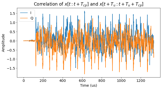
The next figure shows how the correlation looks like in the presence of a frequency error of 2 kHz. The phase of the correlation peaks now should have an angle of -48 degrees, but we can still easily detect the peaks if we take the complex modulus of the correlation.
A detailed look at the first correlation peak (coming back to the case of no frequency error), shows that it is not easy to locate the vertex of the peak precisely, due to the noise. Therefore, the synchronization that we can achieve with this method is not very accurate. Perhaps we will have an error of a few microseconds. The same problem happens with the regular Schmidl & Cox algorithm.
SC-FDMA demodulation
From the coarse time synchronization obtained with the poor man’s Schmidl & Cox, we can now attempt to demodulate the SC-FDMA PUSCH symbols. Demodulation of an SC-FDMA symbol starts in the same way as with any regular OFDM symbol. We take the 2048 samples that we believe are best aligned with the useful time of our symbol, and perform a 2048-point FFT. Now we need to select the \(M\) FFT bins corresponding to the subcarriers occupied by the SC-FDMA symbol and perform an \(M\)-point IFFT. This will give us the \(M\) QPSK (or QAM) symbols carrier in this SC-FDMA symbol.
This all works well when the symbol is perfectly synchronized. However, it doesn’t when there are synchronization errors, so it pays off to invest some time in thinking how these errors affect an SC-FDMA symbol. Roughly speaking, it’s the other way around compared to regular OFDM, due to the extra DFT.
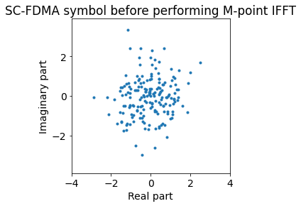
First off, a remark is that it’s impossible to judge synchronization before performing the \(M\)-point IFFT that undoes the precoder action. In fact, if we think about what the precoder does, it takes \(M\) symbols from a QPSK (or QAM) constellation (we can assume that the symbol are randomly chosen), and computes their DFT. The result is close to \(M\) samples taken from uncorrelated complex Gaussian distributions. In this sense, the precoder output looks like AWGN. The figure below demonstrates this by showing the consellation of our first PUSCH symbol before performing the \(M\)-point IFFT. The symbol is in fact perfectly synchronized, but it’s impossible to tell from this plot.
The “hard” way to see how synchronization errors affect SC-FDMA uses the definition in terms of the precoder, and goes like this. First assume we have an STO (symbol time offset). After demodulation of the OFDM symbol, we get a phase vs. frequency slope. Now we perform the \(M\)-point IFFT. This transforms the phase vs. frequency slope into a circular shift of its output. In general, the amount that is shifted will not be an integer number of samples. This means that each QPSK (or QAM) symbol gets mixed with one of its neighbours (actually with all of them, due to how a fractional delay works). This is ISI (inter-symbol interference), and we get a constellation that looks like garbage.
On the other hand, assume that we have a CFO (carrier frequency offset). This means that our demodulation FFT is not well aligned with the OFDM subcarriers. If this were a regular OFDM symbol, the contents of neighbouring subcarriers (which carry different QPSK or QAM symbols) would get mixed by the FFT, and we would get ISI. We can understand the CFO as a fractional shift in the frequency domain, that mixes neighbouring carriers. For an SC-FDMA symbol, this shift in the frequency domain almost gets transformed into a modulation in the time domain after doing the \(M\)-point FFT (the “almost” is because the shift is not cyclic). This modulation is a phase vs. time slope in our final QPSK (or QAM) symbols. This is not as bad as having ISI, and moreover we can measure this slope and use it to estimate and correct the CFO.
I find much easier to arrive at the same conclusions by thinking of SC-FDMA as a time-domain PAM modulation. If we have an STO, then we are going to get ISI unless our STO happens to be close to an integer number of time-domain symbols. Note that the time-domain symbols are rather short, since their duration is \(T_u/M\). In our case, as we will see, the PUSCH signal occupies \(M = 180\) subcarriers, so the time-domain symbol duration is ~0.37 us, or 11.37 samples. If we have a CFO, then the phase of our time domain-symbols PAM symbols changes as we advance in time, so we get a phase vs. time slope from which we can estimate the CFO.
Achieving accurate enough time synchronization by looking at the SC-FDMA PUSCH symbols alone is quite hard. The reason is that while it is easy to ensure that the STO is close to an integer multiple of the time-domain PAM symbol length \(T_u/M\), for otherwise the constellation will have severe ISI and look really bad, it is difficult to ensure that the STO is indeed close to zero, or in other words, that we haven’t slid our synchronization by a few time-domain symbols.
In fact, here the presence of a cyclic prefix doesn’t help. If we slide the synchronization one symbol backwards, we will take the last time-domain symbol of the cyclic prefix as our first symbol. The constellation will be correct and everything will look great except that the QPSK (or QAM) symbols will be circularly shifted by one place. This will be disastrous when we try to interpret the data. If, on the other hand, we slide the synchronization one symbol forwards, then we are dropping the first time-domain symbol and taking the start of the cyclic prefix of the next OFDM symbol as our last time-domain symbol. What happens depends on whether the cyclic prefix length is close to an integer number of time domain symbols (i.e., whether \(T_{cp}M/T_u\) is close to an integer), and whether the next OFDM symbol is actually a PUSCH symbol using the same subcarriers (as it could be a DMRS symbol, for instance). All this will determine whether this last time-domain symbol will be a perfectly valid QPSK (or QAM) symbol extracted from the next PUSCH symbol, an ISI mixture of two QPSK (or QAM) symbols from the next PUSCH symbol, or just garbage.
For these reasons, it is advisable to use the DMRS symbols for fine time synchronization. We will do so below. Otherwise, it is not difficult to get a clean QPSK (or QAM) constellation out of the SC-FDMA PUSCH symbols, but the data could be garbled.
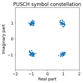
As a demonstration of this discussion on synchronization, the figure below shows the constellation of our first PUSCH symbol when everything is well synchronized. We have also adjusted the amplitude and phase of the signal to get the QPSK symbols in their expected locations.
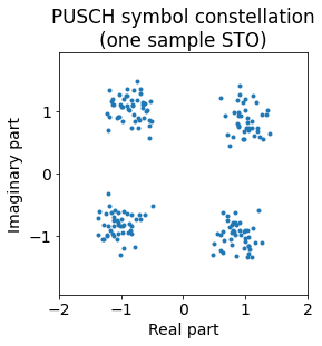
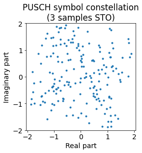
The next figures shows what happens when we introduce just one sample (~0.033 us) of time offset. This is very noticeable, as we start to get significant ISI.
With just 3 samples (~0.098 us) of time offset the ISI is so severe that the constellation is garbage. Recall that time-domain PAM symbols are 11.37 samples long in our case, so here we are looking at a synchronization error of 26% of a time-domain symbol.
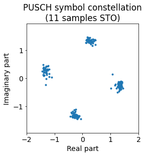
However, if we keep increasing the STO, when we arrive to an offset of 11 samples, which is close to a time-domain PAM symbol, the constellation looks good again. The phase of the constellation has rotated, because the allocation for our subcarriers is not centred at DC, so a time delay also gives us a phase rotation. However, since we do not know the phase of the signal, we can’t use this phase rotation to detect that we’re a time-domain PAM symbol off. This shows clearly that just by looking at the PUSCH symbols we can get a clean QPSK constellation, but not ensure correct time synchronization.
Note that in this case a sample is a relatively small fraction of a time-domain PAM symbol (8.8%), so we are able to obtain good synchronization by using a delay which is an integer number of samples. If the PUSCH signal uses many more subcarriers, then a sample will be a much larger fraction of a time-domain PAM symbol, and we will need to do a fractional sample delay to achieve good synchronization and avoid ISI. The natural way to do this is in the frequency domain, by applying a suitable phase vs. subcarrier slope before performing the \(M\)-point IFFT that undoes the precoder action. It is possible to adjust this fractional delay by looking at how much ISI the constellation has. In our case, we could also use this technique to attempt to improve further our QPSK constellation.
For completeness, let us look now at the effects of a CFO. We come back to a good time synchronization and introduce a CFO of 2 kHz. The constellation looks like this.
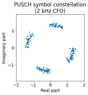
It is easier to see what happens if we plot the phase of each symbol versus the symbol number. We get a phase vs. symbol number slope, which is actually a phase vs. time slope.

From this slope we could estimate the 2 kHz CFO and correct it. This would work even if we have an error in the time synchronization that is close to an integer multiple of time-domain PAM symbols. We could even look at several consecutive SC-FDMA PUSCH symbols to measure the phase drift over a longer time span and thus estimate and correct the CFO very precisely. The conclusion is that even though looking at the PUSCH symbols alone it is very difficult to estimate and correct the STO, on the other hand, it is easy to estimate and correct the CFO.
There is still a matter related to the demodulation of the PUSCH symbols that we haven’t treated so far. This is how to determine which subcarriers are in use. In principle, this could be determined from the PSD of the signal, by looking at where its edges are. It is rather easy to determine the number of subcarriers in use, because the allocation must be a whole number of RBs (resource blocks), that is, an integer multiple of 12 subcarriers. Since an RB is 180 kHz wide, it is very easy to count RBs in the waterfall, for instance in inspectrum, without making mistakes. In some of the figures above we can see that the signal we are analysing is about 2.7 MHz wide, so that is 15 RBs, or 180 subcarriers.
Now, unless we are looking at a “high-resolution” PSD that can tell us where the edges of the signal are with a precision on the order of a few kHz (so we’d better use several symbols to produce this PSD, as otherwise the resolution will not be good enough), it is easy to make a mistake and “slide off” by a few subcarriers in our choice of the 180 active subcarriers. What happens if we do so? The first remark is that some of the subcarriers will only contain noise, so their amplitudes will be small compared to those of the good subcarriers. However, if the CFO is significantly high (for instance, say 20% of the subcarrier spacing), then one of our subcarriers will contain a fraction of a good subcarrier, so its amplitude will not be as small as if it only had noise.
Moreover, if we are looking at SC-FDMA symbols, as we have seen, before undoing the precoder the symbols carried in the OFDMA subcarriers resemble AWGN. This means that their amplitude could be small, so we could mistake the outermost subcarriers for noise. A similar thing may happen with a QAM OFDMA constellation, specially if the constellation order is high. All this means that depending on the circumstances, it is possible to make a mistake and end up sliding off by just one subcarrier.
The effects of this mistake on regular OFDM symbols are not so obvious, since only one of the subcarriers is affected. However, the effects on SC-FDMA symbols are very obvious. In fact, to the time-domain PAM symbols the mistake looks exactly like a phase vs. time slope produced by a CFO of 15 kHz. Therefore, the PUSCH symbols are quite helpful to check that we have select the appropriate subset of subcarriers.
An illustration of this discussion is given by the next figure, which shows the amplitudes of the OFDMA subcarriers of a PUSCH symbol (before applying the precoder). Only the frequency span surrounding our PUSCH allocation is shown. It is clear that the outermost OFDMA subcarriers are very small and contain only noise. However, if we try to tell where are exactly the edges of the PUSCH allocation, we can run into trouble, because sometimes we are not sure if we’re looking at a precoded SC-FDMA symbol that just happens to be small, or to a subcarrier than only has noise. In this figure there is no CFO, but the situation would be even more difficult with a relatively large CFO.
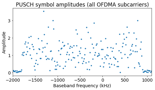
In our case, the PUSCH symbols occupy the OFDMA subcarriers numbered from 905 to 1084. Taking into account that we have arranged things so that the OFDMA subcarrier at DC (which has number 1024) corresponds to the uplink subcarrier at a frequency of -7.5 kHz, we see that PUSCH allocation occupies from the subcarrier at -1792.5 kHz to the subcarrier at 892.5 kHz.
Something we haven’t used to our advantage while finding which subcarriers are occupied by our signal is that the RB frequency grid is fixed, in the following sense. There are two RBs, whose edges are at 0 Hz. One of them encompasses subcarriers centred from +7.5 kHz to +187.5 kHz, while the other encompasses subcarriers centred from -187.5 kHz to -7.5 kHz. The remaining RBs in the grid are obtained by adding an integer multiple of 180 kHz to these. Knowledge of this fact can help us avoid the mistake of being “one subcarrier off”, since that wouldn’t be aligned to the RB grid. However, this would only work if our initial CFO is smaller than the subcarrier spacing.
In our case, we see that the PUSCH signal occupies 5 RBs to the right of 0 Hz and 10 RBs to the left of 0 Hz, making up the total 15 RBs. Moreover, after working carefully with the PUSCH symbols as described above, we can see that the CFO in the recording is around 1560 Hz. This is 1.84 ppm, so it is on the ballpark of what we expected.
Demodulation of the PUSCH and DMRS symbols
In the previous section we have seen how to use the PUSCH symbols to obtain time and frequency synchronization, with the only caveat that we may be off in the time synchronization by an integer number of time-domain PAM symbols, which causes a good PUSCH constellation but potentially garbled data. We can also adjust the phase and amplitude of the signal by looking at the PUSCH constellation, especially when it is a simple constellation such as QPSK (albeit we will have a 90º phase ambiguity that really needs to be sorted out with the DMRS).
Below we will see how to make use of the DMRS to obtain good synchronization, but even so, at this moment we can already demodulate all the symbols in the 14 slots (7 ms) that we are analysing in this post. The only things that we need to take into account is where the first symbol starts, the fact that the cyclic prefix of the first symbol in each 7-symbol slot is slightly longer, and the fact that the middle symbol in each slot belongs to the DMRS, so we shouldn’t apply the \(M\)-point IFFT to it.
With these things in mind, we can obtain a figure like the one below, where the constellations of the 7 symbols in each slot are shown in a row of the table. The middle symbol in each slot corresponds to the DMRS, which as we will describe is an OFDMA symbol that contains symbols from a Zadoff-Chu sequence. This sequence is formed by complex numbers of modulus one that are spread over all the unit circle. This explains why the constellation looks that way. This also means that the DMRS is not helpful to assess time or frequency synchronization unless we “wipe off” the Zadoff-Chu sequence, which we will do below.
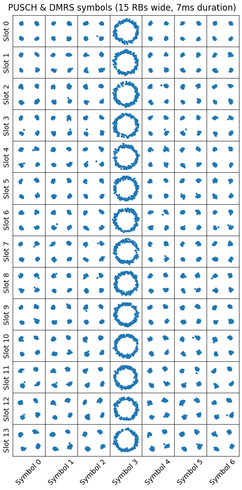
We see that the QPSK constellation of the PUSCH symbols looks quite good all the time. We can see that by the last symbols it has rotated slightly. This may be due to a CFO, but also to a SFO (sample frequency offset). When there is an SFO, it will cause an monotonically increasing or decreasing time delay. If the OFDMA allocation is not centred at DC, this in turn will cause a monotonically increasing or decreasing phase error. We will look at this in more detail with the help of the DMRS.
Zadoff-Chu sequences
Zadoff-Chu sequences are used to construct the DMRS, as well as other pilot signals in LTE. Here we will define them only in the generality that is needed for the most common LTE scenarios, since Zadoff-Chu sequences can be defined in a more general way, as for instance is done in Wikipedia. We follow the notation of Section 5.5.1.1 in 3GPP TS 36.211.
If \(N_{ZC}\) is an odd prime and the integer \(q\) satisfies\[q \not \equiv 0 \mod N_{ZC},\] the Zadoff-Chu sequence \(x_q(m)\) is defined as\[x_q(m) = \mathrm{exp}\left(-\frac{i\pi q m (m+1)}{N_{ZC}}\right),\quad m \in \mathbb{Z}.\]Note that this definition only depends on the conjugacy class of \(q\) modulo \(N_{ZC}\), since \(m(m+1)\) is even for all \(m\).
The first property of this sequence is that it is \(N_{ZC}\)-periodic. This is a consequence of the fact that\[(m+kN_{ZC})(m+kN_{ZC}+1) – m(m+1) = (2m+1 + kN_{ZC})kN_{ZC}\]is always an even multiple of \(N_{ZC}\) for every \(m, k\in \mathbb{Z}\), because \(N_{ZC}\) is odd.
One way to think of the Zadoff-Chu sequence \(x_q(m)\) is as a chirp whose instantaneous frequency is \(-q(m+1)/N_{ZC}\) cycles/sample, because \((m+1)(m+2)-m(m+1) = 2(m+1)\). We get aliasing, so we can think of reducing \(q(m+1)/N_{ZC}\) modulo 1 to give something between -1/2 and 1/2 cycles/sample.
A nice property of Zadoff-Chu sequences is that the DFT of the sequence \((x_q(m))_{m=0}^{N_{ZC}-1}\) is given by \((\lambda \overline{x_{q^{-1}}(m)})_{m=0}^{N_{ZC}-1}\), where \(q^{-1}\) denotes the multiplicative inverse of \(q\) modulo \(N_{ZC}\), and \(\lambda\) is whatever constant factor we need for Parseval’s theorem to hold depending on our definition of the DFT (in particular, \(\lambda = 1\) if we use the unitary DFT). This was proved in the 2009 paper Efficient computation of DFT of Zadoff-Chu sequences, even though Zadoff-Chu sequences have been studied since the 70s at least. In hindsight, this result is not so surprising if we think of Zadoff-Chu sequences as chirps. If we interchange the time and frequency domains of a chirp, we get another chirp. What is interesting is that we still get a chirp of the particular form that Zadoff-Chu sequences have, and that the structure of the multiplicative group of the field \(\mathbb{Z}/N_{ZC}\mathbb{Z}\) is somehow behind this transposition of the time and frequency axes.
In this paper, the result was proved mainly with the interest of giving a more efficient way of computing the time-domain LTE symbols that involve Zadoff-Chu sequences, since the naïve way would involve computing the Zadoff-Chu sequence that corresponds to the frequency-domain symbols and then computing their IFFT. However, this relation also gives a very simple way to prove two important properties of Zadoff-Chu sequences.
The first of these properties is that the circular autocorrelation function of \((x_q(m))_{m=0}^{N_{ZC}-1}\) is zero except at lag zero. To see this, we use the convolution theorem to compute the autocorrelation in the frequency domain. We see that the PSD of our Zadoff-Chu sequence is given by \((\lambda^2 |x_{q^{-1}}(m)|^2)_{m=0}^{N_{ZC}-1}\). This is constant in \(m\), so its inverse DFT is a Dirac delta at the origin.
The second property is that if \(q_1 \neq q_2\), then the circular cross-correlation of \((x_{q_1}(m))_{m=0}^{N_{ZC}-1}\) and \((x_{q_2}(m))_{m=0}^{N_{ZC}-1}\), defined as\[\sum_{k=0}^{N_{ZC}-1} x_{q_1}(m+k) \overline{x_{q_2}(k)},\]has constant modulus \(\sqrt{N_{ZC}}\). Working in the frequency domain as above, we find that the DFT of this cross-correlation is\[\lambda^2\overline{x_{q_1^{-1}}}(m)x_{q_2^{-1}}(m) = \lambda^2 x_{q_2^{-1}-q_1^{-1}}(m).\] In order for the usual formula of the convolution theorem to hold, we must use the non-unitary DFT. In this case, \(\lambda =\sqrt{N_{ZC}}\). Applying the inverse DFT to the right-hand side of the equality above, we get\[\lambda \overline{x_{(q_2^{-1}-q_1^{-1})^{-1}}(-m).}\]This has constant modulus \(\sqrt{N_{ZC}}\).
The DMRS symbol
The definition of the PUSCH DMRS symbol is given in several subsections of Section 5.5 in TS 36.211. This LTE quick reference page gives a good summary of the formulas involved. The symbol is constructed from a Zadoff-Chu sequence in the following way. We denote by \(M\) the number of subcarriers occupied by our PUSCH uplink, and assume that at least 3 RBs are used, so that \(M \geq 36\). We choose as \(N_{ZC}\) the largest prime smaller than \(M\). Two integer parameters \(0\leq u \leq 29\) and \(v=0,1\) are used to choose \(q\) acccording to the following relations:\[\overline{q} =\frac{N_{ZC}(u+1)}{31},\]\[q = \lfloor\overline{q}+1/2\rfloor + (-1)^{\lfloor 2\overline{q}\rfloor}v.\]Note that \(1 < \overline{q} < N_{ZC}-1\), which implies \(1 \leq q \leq N_{ZC}-1\), so that \(q\) is not congruent to zero modulo \(N_{ZC}\) (to see this, when \(v = 1\) the cases \(\overline{q} \in [1, 3/2)\) and \(\overline{q} \in [N_{ZC}-3/2, N_{ZC}-1)\) need to be examined with some care to determine the value of the term \((-1)^{\lfloor 2\overline{q}\rfloor}\)). Additionally, a number \(\alpha\) of the form \(\alpha = 2\pi n_0/12\), \(n_0\in\mathbb{Z}\) is chosen.
The DMRS symbol is an OFDMA symbol whose subcarriers transmit the following sequence of complex numbers of modulus one:\[r(n) = e^{i\alpha n}x_q(n),\quad n=0,1,\ldots,M-1.\]Here I have made some simplifications with respect to the full generality of TS 36.211. This simplified description still matches the signal we are analysing.
The building block for \(r(n)\) is the Zadoff-Chu sequence \(x_q\). Since \(M\) is slightly larger than \(N_{ZC}\), the sequence \(r(n)\) contains slightly more than one period of \(x_q\). In our case, since the PUSCH occupies 15 RBs, we have \(M = 180\), so \(N_{ZC} = 179\), and we use one period of \(x_q\) followed the first element again.
The term \(e^{i\alpha n}\) is referred to in TS 36.211 as a cyclic shift. The way to understand this is that the values \(x_q(n)\) form the subcarriers an OFDMA symbol, so they are in the frequency domain. A multiplication by \(e^{i\alpha n}\) in the frequency domain is equivalent to a cyclic shift in the time domain. In fact, the effect of this multiplication is to perform a time-domain cyclic shift to the useful symbol by some integer multiple of \(T_u/12\) (given by the value of \(\alpha\)). Note that it is the useful symbol the one which is shifted cyclically. The cyclic prefix is then chosen accordingly.
The parameters \(u\), \(v\) and \(\alpha\) to use for each DMRS symbol are determined from some parameters of the higher protocol layers. I haven’t understood very well how this works, but I think the eNodeB always knows what parameters to expect due to its previous communications with the UE. However, in our case we do not know a priori the values for \(u\), \(v\) and \(\alpha\). The parameters \(u\) and \(v\) may change in each slot when group hopping or sequence hopping are enabled, or they may be maintained for some time (which is what happens with our signal). The parameter \(\alpha\) changes in each slot, however.
Finding the DMRS parameters
We need a way to find the DMRS parameters \(u\), \(v\) and \(\alpha\) that the UE is using in our recording. The method we choose should work in the presence of some STO. The effect of STO on the sequence of DMRS OFDMA subcarriers is the multiplication by \(e^{i\beta n}\) for some \(\beta\). We can group this effect with the shift \(e^{i\alpha n}\).
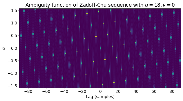
Considering the ambiguity function of \((x_q(n))_{n=0}^{M-1}\) is a good idea. This function is defined by\[A(\alpha, k) = \frac{1}{M}\sum_{n=0}^{M-1} e^{i\alpha (n+k)} x_q(n+k \operatorname{mod} M) \overline{x_q(n)},\quad \alpha\in\mathbb{R}, k \in \mathbb{Z}.\]This gives the cross-correlation of frequency shifted versions of \(x_q\), and \(x_q\) itself. It turns out that for each \(\alpha\), there is some \(k\) (depending on \(\alpha\)) such that \(A(\alpha, k)\) is relatively large (larger than approximately \(1/2\)). Moreover, the cross-ambiguity function\[A_{q_1,q_2}(\alpha, k) = \frac{1}{M}\sum_{n=0}^{M-1} e^{i\alpha (n+k)} x_{q_2}(n+k \operatorname{mod} M) \overline{x_{q_2}(n)}\]is small if \(q_1 \not\equiv q_2 \operatorname{mod} N_{ZC}\). I haven’t tried to prove these facts, but numerical simulations support them. They are somewhat intuitive if we think of \(x_q(n)\) as a chirp and of \(q\) as its slew rate, since chirps have this property about their ambiguity functions (a frequency shift of a chirp correlates with a time translation of said chirp), while chirps with different slew rates don’t correlate even if we allow performing frequency shifts.
As an illustration, the figure below shows the ambiguity function of \((x_q(n))_{n=0}^{M-1}\) for the Zadoff-Chu sequence corresponding to our signal, which as we will see below uses the parameters \(u = 18\), \(v = 0\). This doesn’t look very much like the prototypical ambiguity function of a chirp in continuous time, which is a set of diagonal lines, but the reason is that the slew rate of Zadoff-Chu sequences is quite large and immediately gives rise to aliasing.
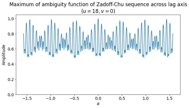
The next figure shows, for each \(\alpha\), the value of \(\max_k A(\alpha, k)\). This maximum never goes below approximately 0.5. It is interesting to compare this plot with the ambiguity function to try to see where the maximum is attained in each case.
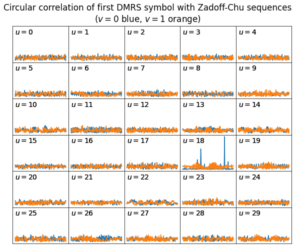
This discussion motivates a way to find the DMRS parameters \(u\) and \(v\). We can forget momentarily about \(\alpha\) and any possible STO. We consider all the possible values of \(u\) and \(v\) (there are 60 combinations) and the sequences \((x_q(n))_{n=0}^{M-1}\) that each of them gives rise to. If we denote by \((r(n))_{n=0}^{M-1}\) the values of the OFDMA subcarriers of one of our DMRS symbols, we can compute the circular cross-correlations of \((r(n))\) and each of the sequences \((x_q(n))\). These circular cross-correlations can be evaluated efficiently by means of the FFT. According to the properties of \(A_{q_1,q_2}\) given above, the cross-correlation corresponding to the correct values of \(u\) and \(v\) will have a large amplitude for some lag, while the others will be small.
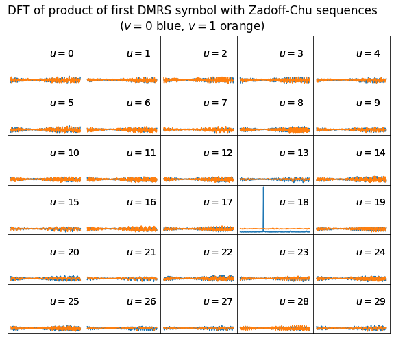
The next figure shows the results of applying this procedure to the first DMRS symbol in our signal. The scale for all the plots is the same. We can see clear cross-correlation peaks in the plot corresponding to \(u = 18\), \(v = 0\), while the remaining plots have small amplitude.
An alternative approach which is perhaps simpler and more efficient is as follows. Instead of considering the cross-ambiguity function \(A_{q_1,q_2}\), we consider the product\[\Pi_{q_1,q_2}(\alpha, n) = e^{i\alpha n}x_{q_1}(n) \overline{x_{q_2}(n)}.\]If \(q_1 \equiv q_2 \operatorname{mod} N_{ZC}\), then this product is just \(e^{i\alpha n}\), so when we take its DFT we will see a large peak at the frequency \(\alpha\). On the other hand, if \(q_1 \not\equiv q_2\operatorname{mod}N_{ZC}\), then\[\Pi_{q_1,q_2}(\alpha, n) = e^{i\alpha n}x_{q_1-q_2}(n).\]The DFT of this is essentially a circularly shifted version of the DFT of \((x_{q_1-q_2}(n))_{n=0}^{M-1}\). Above we have seen that the DFT of a Zadoff-Chu sequence taken over a period of \(N_{ZC}\) samples is essentially another Zadoff-Chu sequence. In particular, it has constant amplitude, which means that the power is spread over all the DFT bins, instead of being concentrated in a single bin (note that we always have \(|\Pi_{q_1,q_2}(\alpha, n)| = 1\), so the total power is always the same). In this case we are taking a DFT over \(M\) samples, which is somewhat longer than \(N_{ZC}\). However, the results are similar. The power of the DFT of \(\Pi_{q_1,q_2}\) is spread more or less equally over all the DFT bins.
The figure below shows the results of applying this procedure to our first DMRS symbol. We can see the large peak in the correct Zadoff-Chu sequence. The other Zadoff-Chu sequences spread the power over all the DFT bins.
Once we have found the parameters \(u\) and \(v\), it is straightforward to find the parameter \(\alpha\) corresponding to the frequency term \(e^{i\alpha n}\). However, since we have STO, we are in fact seeing \(e^{i(\alpha+\beta) n}\), where \(\beta = 2\pi\Delta t/T_u\) and \(\Delta t\) denotes the STO. Therefore, we need to have \(|\Delta t| < T_u/24\), since otherwise part of the STO would be mistaken as forming part of \(\alpha\) (recall that the possible cyclic shifts corresponding to \(\alpha\) are spaced \(T_u/12\)). This time synchronization is easy to achieve by using the poor man’s Schmidl & Cox method introduced at the beginning of the post.
DMRS amplitude and phase
Once we have found the parameters \(u = 18\) and \(v = 0\), which in our case do not change in the 7 ms of signal we are analysing, and \(\alpha\), which changes in each slot, we can multiply the demodulated OFDMA DRMS symbols with the correct reference sequence to obtain the phase of each subcarrier. We can also measure the amplitude of each subcarrier, though for this it is not necessary to use the reference sequence, since it has constant modulus one.
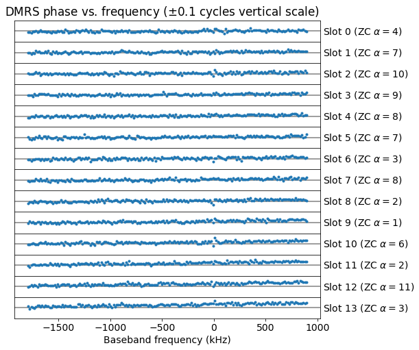
While doing this I have observed something that I haven’t been able to find in the 3GPP documentation. In the odd slots, the DMRS symbol is multiplied by -1 (Or maybe in the even slots. I can’t tell, since I haven’t stablished an absolute phase reference for the signal). What is clear is that if I just multiply by the received symbols by the complex conjugate of the DMRS reference sequence computed as described above, then the phase of the subcarriers will jump by 180 degrees every other symbol. I have tried to search for some mention of this “change of sign” of the DMRS, but haven’t found anything similar.
The figure below shows the phase versus frequency of the DMRS subcarriers, after taking into account and correcting this “change of sign”. The parameter \(\alpha\) used in each slot is shown as the integer \(n_0\) such that \(\alpha = 2\pi n_0/12\). Using this figure we can estimate and correct for the STO (which will cause a slope in phase versus frequency) and also estimate and correct the phase (though we had already done that using the QPSK PUSCH symbols, those have a 90º ambiguity).
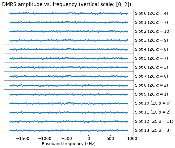
The plot of the amplitude versus frequency is shown below. As expected, the amplitude is flat, since there is no multipath in this recording. Also, the amplitude is close to one, since we had already adjusted the amplitude by using the QPSK PUSCH symbols.
Equalization
The equalization of the signal in this recording is quite easy, because there is no multipath. We only need to correct the STO and carrier phase offset. To do this, we first estimate them using the phase versus frequency measurements of the DMRS symbols. By fitting a polynomial of order one to these measurements, we can get the STO as the order one coefficient and the carrier phase as the order zero coefficient. When doing this, we need to take into account that the PUSCH allocation is not at baseband, but rather centred at around -450 kHz. We need to consider baseband frequency as the independent variable of this polynomial.
The next figure shows the phase and delay measurements obtained from the DMRS symbols. We see that the phase starts close to zero, because we have already adjusted the phase of the signal according to the first DMRS symbol. However, the phase then increases slightly, and at symbol 8 it starts increasing steadily. This is due to a change in CFO.
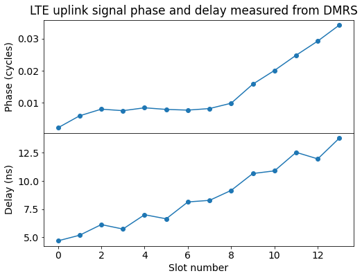
Besides this, we also see that the delay keeps increasing steadily throughout the 7 ms of signal that we are analysing. This is caused by an SFO. If left uncorrected, the change in delay will eventually cause a large phase rotation for the carriers which are away from baseband. However, a delay of 10 ns gives a phase rotation of 0.01 cycles to a subcarrier that is 1 MHz away from baseband. This means that most of the phase rotation that we saw in the QPSK symbols of the last slots comes from the carrier phase offset rather than from the STO.
We also take the average amplitude of the DMRS symbol of each slot to equalize the amplitude of the signal, though it only changes very slightly over the course of our 14 symbols. Using the all this data, we can now equalize our QPSK PUSCH symbols, obtaining the plot below. The ideal locations for the symbols are plotted as small red dots.
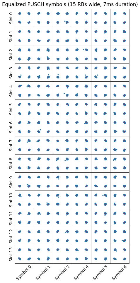
We can use the equalized constellation to measure the EVM (error vector magnitude) of the signal. This is the RMS error between the received and ideal QPSK constellation symbols, divided by the amplitude of the ideal symbols, which is \(\sqrt{2}\). For the PUSCH symbols we have demodulated, the EVM is 8.6%, or -21.3 dB.
Code and data
The code used to process the signal and make the plots shown in this post is in this Jupyter notebook. The signal analysed here is an extract of the the LTE_uplink_847MHz_2022-01-30_30720ksps SigMF file, which can be found in this location.
Update 2023-09-27: I have updated the Jupyter notebook to handle the 7.5 kHz uplink subcarrier offset correctly. By doing this, the sign change in every other DMRS does not appear. For more details see the “Symbol inversion” section in the next post and this comment.
Hi,
I am just wondering if you could decode the phone number?
Thanks.
regards,
chin
I don’t know. It’s probably buried under several protocol layers and encrypted.
May I ask a question how did you compute CFO and the time offset correction from DMRS?
See cell [23] in the notebook.
I agree that the cell 23 is plotting something related to CFO. Would you mind explain more details how to obtain the values from the figures, CFO= 1560Hz, time offset correction from DMRS=-44?
Hi Daniel,
Thanks again for your continued good work. Can you answer a few questions?
1. How would the analysis/processing change if the modulation was 16 or 64 QAM instead of QPSK? Will your code/plots still work for these modulation schemes too?
2. I recorded some UL signals transmitted by srsRAN enabled eNB and received using Pluto SDR. I used Matlab toolbox to find the timing offset, freq offset and corrected them. Next I use your Python code for subsequent processing. The SNR is above 10 dB as the SDRs are placed close together. However, OFDM subcarriers amplitudes are low owing to which I could not extract which subcarriers are in use. Also, the resultant constellation is quite bad with all points gathered around the center. Any thoughts?
Hi Sohail,
1. Nothing done here uses QPSK in a very specific way, so it should also work for 16 and 64 QAM.
2. I don’t understand exactly the problem. You say that the SNR is good but the amplitude is low. Can’t you just multiply the IQ data by a constant to normalize the amplitude? In the Jupyter notebook for this post this is done in cell [2] (the division by 2e4).
Many thanks again, Daniel. I’ll look at your Jupyter notebook again.
Sohail,
Did you succeed in demodulating your captures using plutoSDR?
Do you have a possibility to share your IQ files?
Is the demodulation of symbol3 (Zadoff-chu) essential? Can’t we interpret the signal in the frequency domain to estimate the channel and equalize it?
It is an OFDM symbol after all, so the most natural way of treating it is as such. What do you mean precisely by “interpret the signal in the frequency domain”?
If I look at each slot, the ZC sequence seems to occupy most of the subcarriers(FFT length) in symbol3. What is the difference between the designated positioned Pilot Carrier (eg. if occupied_carriers = ((1, 2, 3), (1, 2, 4))) and this ZC Sequence type?
I don’t understand what you’re talking about. Perhaps it’s something different from the PUSCH DMRS? Can you give a reference to these pilot carriers and occupied carriers?
For example, 802.11a/g reserves four(Out of 52 populated subcarriers) to be used as “pilot subcarriers”, which are used for channel estimation and synchronization between transmitter and receiver. But this ZC sequence(Pilot Symbol) seems to occupy most of the subcarriers(FFT length) in symbol3. I wonder what the difference is between the two methods and whether they are terminally different..
(https://www.wirelesstrainingsolutions.com/understanding-ofdm-part-2-refresh/) this link is 802.11 OFDM
The approaches are somewhat different. The PUSCH DMRS occupies all the subcarriers allocated to the PUSCH transmission. It uses a ZC sequence in the frequency domain so that it also has constant envelope (or nearly constant; I don’t remember well) in the time domain, due to the interesting properties of the ZC sequences. This is in-line with the SC-FDMA modulation of the PUSCH also having low PAPR, although the DMRS is a regular OFDM symbol, not SC-FDMA.
Hi Daniel,
One more question. I see that you have performed fine frequency offset estimation using DMRS symbols. Another but simpler method that I have seen in research papers [e.g. Eq 5 of https://www.researchgate.net/publication/4296407_Frequency_Offset_Estimation_for_High_Speed_Users_in_E-UTRA_Uplink%5D is to employ correlation between two DMRS symbols in one subframe (4th and 11th symbols; index 3 and 10), since they are essentially same, if there is no hopping. I employed that method but it does not give me the same result as yours. Any comments you can offer? Thanks
Hi Sohail, why do you say that the two DMRS in a subframe are essentially the same? If you look at the plot https://destevez.net/wp-content/uploads/2022/02/dmrs_phase.png, you’ll see that the parameter α keeps changing every slot. Maybe there is hopping in this case? I don’t remember the details of how the sequence of α’s is chose off the top of my head.
Thanks for the reply. Some papers I read state that in case of no hopping, these DMRS symbols are same. Thus, they act like pilot symbols which can be used for channel estimation and frequency estimation purposes. I’ll dig deeper into this.
Also, can you offer any key points to remember when recording UL signal? I’m not sure but I guess I’m not recording the correct PUSCH signal; my signal and its spectrum looks different from yours and that of the UL signal generated in MATLAB. Any pics of your experimental setup would help, if it is no trouble and waste of your time. Thanks again for your time.
The recording set up for this was really simple. I put my phone on top of a B205mini (with metal case). The B205mini had no antennas connected. I played a Youtube video on the phone to generate some traffic. I used GNU Radio to record at 30.72 Msps.
Great. Thanks. You are always prompt and helpful.
Kind regards.
Hello. I sound about SRS signal in uplink of LTE can u tell me is always that is there in uplink frame or its optional signal?. Thanks
I don’t know exactly under which conditions the SRS is transmitted, but for instance there doesn’t seem to be an SRS transmission in this uplink recording.
thanks for your answer. i am working on positioning and now i need real signal of LTE but my device is bladerf and i run in ubuntu SRSRAN can u please help me how can i have a sigMF capture with that device ?
my next question is for example you captured here data for example DMRS part i want to know is this signal that affected by pathloss and fading or by equalization and estimation stage omitted from signal?
thanks
You can record from the BladeRF using GNU Radio’s File Sink (this will be the .sigmf-data file) and then create the .sigmf-meta file using the SigMF Python library. I don’t quite understand your second question.
because of i need to users position in a local LTE network i have to use SRSRAN project to connect users to my semi eNB and EPC so then i use their signal and i dont need to other users in that location. any way thanks for your help. i am very thankful from u to answer the questions when i asked questions in other sites they didnt attention.
What a fantastic post, this was a great help when I was trying to do the same thing!
One correction, I believe that the 1/2 carrier shift should be -7.5 kHz, not +7.5 kHz. If you look at 36.211 5.6, you can see they add 1/2 bin to the output waveform, so the output is 7.5 kHz higher. In your case, the difference was absorbed by the unknown offset of the b200 (which can be large).
The other thing to note, is that I too saw the strange inversion of the second DM-RS symbol. After a lot of messing around I determined that the only way to get the CRC to pass was to invert every second symbol. I cannot explain this, will let you know if I figure it out! It is likely buried in a dangling clause somewhere in 36.211.
Regarding the inversion of every other symbol, I already wrote about this in detail in the next post (https://destevez.net/2022/03/demodulation-of-lte-pucch/). See the “Symbol inversion” section. It has a lot to do with this 7.5 kHz offset.
Reviewing this, I see that I explained all the math in that section, but I never fixed the Jupyter notebooks to handle the 7.5 kHz offset properly (perhaps because I was eager to move of to doing some downlink analysis). Since it seems that these posts are a popular resource and people keep finding them and using them, to avoid confusion I have now modified the Jupyter notebooks to handle the 7.5 kHz offset correctly. With this correction, an inversion of every other symbol is no longer needed, and the CFO is measured correctly (it turns out to be 1060 Hz in this recording).
This is possibly the best reference on LTE UL I have come across. Please keep the great work on.
Could you please answer a query:
How did you arrive at the Selection of subcarriers in use for the part of the capture (i.e from 905 to 1085 -> M =180)
Thank you.
Hello Deepak, I looked at the output of FFT used for OFDM demodulation and selected the subcarriers that had power well above the noise floor.
Thank you!.
I also noticed that the post has the relevant information as well.
Oh Never mind. Let me read the post in more detail.
Hello Daniel, I’m starting working on channel sounding and I find your materials very useful (what I expressed in a small donation:)).
1) Did you comment in your description following lines from the second cell of the notebook?
# Correct for CFO. The CFO is measured with the PUSCH and DMRS.
delta_f = -1060
# Adjust phase offset (done with DMRS signal)
delta_phi = -1.9
2) The waterfall image you showed indicates 2.7 M band.
Also “15 RB * 12 Subcariers * 15 KHz” gives 2.7 MHz band.
However FFT of the 2048 samples from the signal indicates 1.8MHz band.
Please see my notebook on github: https://github.com/MiroslawZoladz/Nokia_ChSounding_DEstevez/blob/master/LTE_Upliknk_demodulation.ipynb
Where am I going wrong?
Hi,
1) Yes. In the post I comment how to find the CFO and carrier phase offset by hand.
2) In your notebook you’re taking the real part of the signal: “fft_roi = fft.fft(np.real(x_roi))”. The signal occupies approximately from -1.8 MHz to +0.9 MHz, so its real part occupies from -1.8 MHz to +1.8 MHz. This is what you see in your FFT.
Many thanks for the details, very helpful but needs time and modelling to follow.
One question: if Zadoff Chu is circular when generated at UE why should we expect it to be equalised as qpsk at receiver.
Sorry I realised symbol3 is not included after equaliser
Can you please elaborate more on how did you get these figures:
delta_f = -1060
delta_phi = -1.9
correction -44 for first sample
Thanks
Hello honorable Daniel Estevez,
Regarding the first big burst of PUSCH seen at 7ms mark – how do you think the scheduling was done for it?
Was there a sequence of DCI format 0 messages at PDCCH, in subframes n-4 for each subframe?
And before that was a ‘Buffer status report’ that signaled the required bits to send?
That is a great question. You might be interested in reading https://destevez.net/2024/06/lte-uplink-pusch/, where I decoded each of the PUSCH transmissions in this decoding to a PCAP file that can be read with Wireshark.
The first “big” PUSCH is packet 14 in the PCAP. 8 ms earlier a “small” PUSCH packet is transmitted. This is packet 11 in the PCAP. It contains a BSR that gives 1817 < BS <= 2127. What is going on is that the UE is transmitting a large (2164 byte) PDCP PDU, which takes a total of 21 subframes to be sent. We don't know exactly what the eNB transmitted (we only have indirect evidence), but it is logical that when receiving the "large" BSR, the eNB decided to allocate more radio resources to the UE. The effects of this are seen 8 ms later (the usual HARQ RTT). I believe there would have been DCI messages in the PDCCH 4 ms before each of these subframes in order to give the uplink grants.