In February this year, the orientation of the orbit of DSLWP-B around the Moon was such that, when viewed from the Earth, it passed behind the Moon on every orbit. This opened up the possibility for recording the signal of DSLWP-B as it hid behind the Moon, thus blocking the line of sight path. The physical effect that can be observed in such events is that of diffraction. The power of the received signal doesn’t drop down to zero in a brick-wall fashion just after the line of sight is blocked, but rather behaves in an oscillatory fashion, forming the so called diffraction fringes.
The signal from DSLWP-B was observed and recorded at the Dwingeloo 25m radiotelescope for three days in February: 4th, 13th and 15th. During the first two days, an SSDV transmission was commanded several minutes before DSLWP-B hid behind the Moon, so as to guarantee a continuous signal at 436.4MHz to observe the variations in signal power as DSLWP-B went behind the Moon. On the 15th, the occultation was especially brief, lasting only 28 minutes. Thus, DSLWP-B was commanded to transmit continuously before hiding behind the Moon. This enabled us to also observe the end of the occultation, since DSLWP-B continued transmitting when it exited from behind the Moon. This is an analysis of the recordings made at Dwingeloo.
The recordings can be found here. I have used my Moonbounce processing scripts to compute the signal power from the recordings. These scripts were made to study the power of the Moonbounce signal, but can be used here as well. Essentially, the script performs Doppler correction using the tracking files published in dslwp_dev as orbit state vector and GMAT as propagator, detects the frequency offset of the GMSK signal from DSLWP-B, lowpass filters it, and takes averaged power readings in windows of 102.4ms.
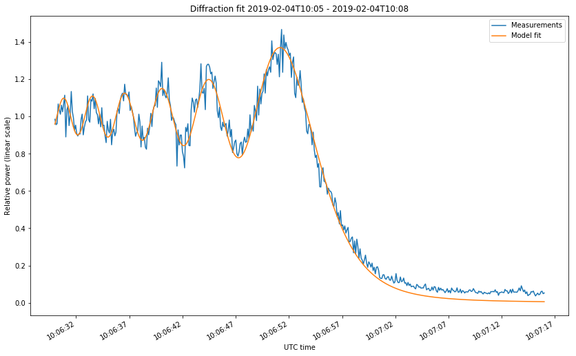
The occultations were planned as shown in this post. After computing the expected times of the occultations, the relevant segments of the power readings are plotted, obtaining the figures shown below.
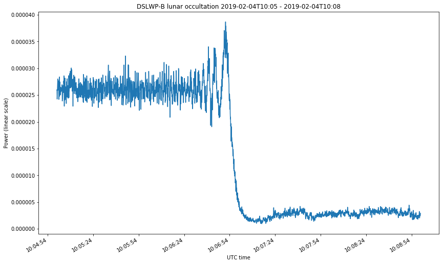
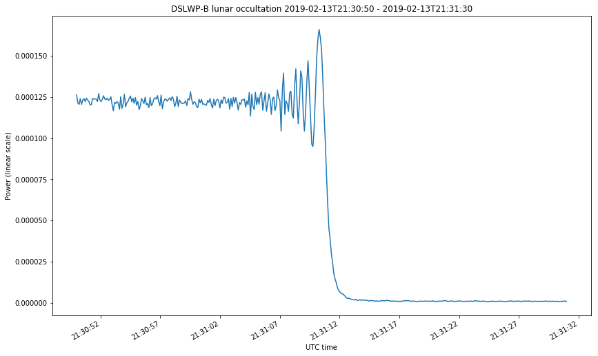
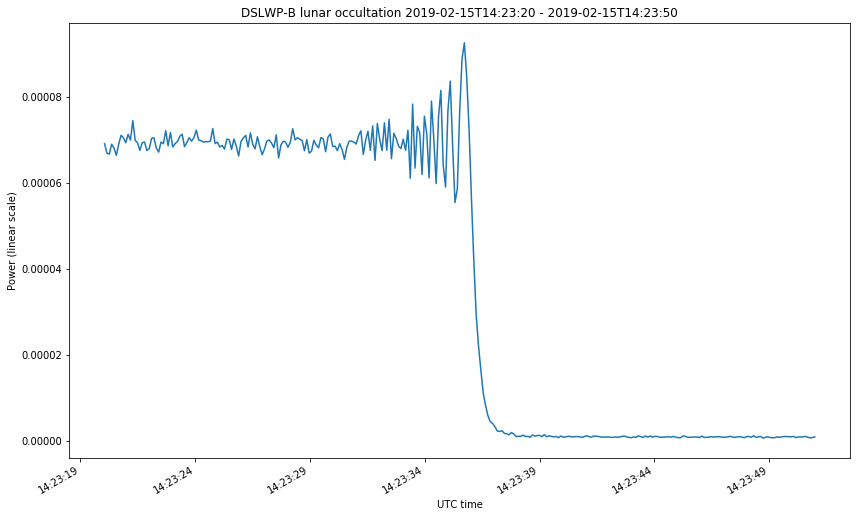
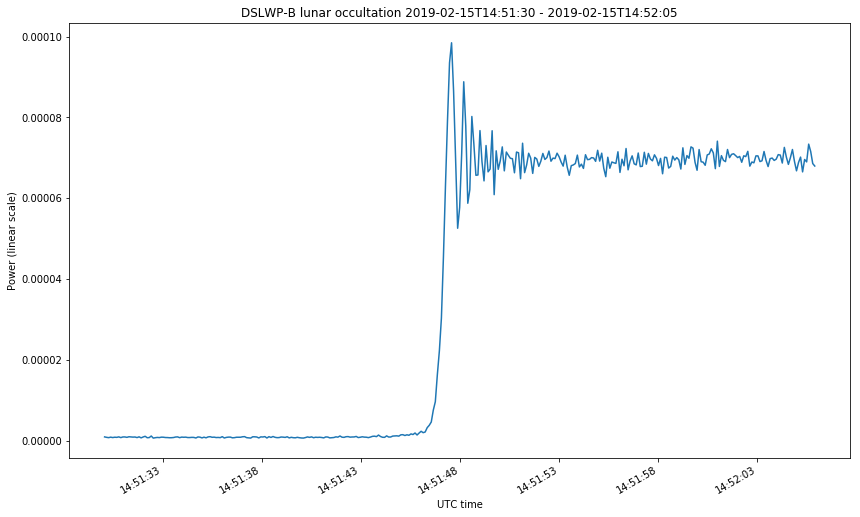
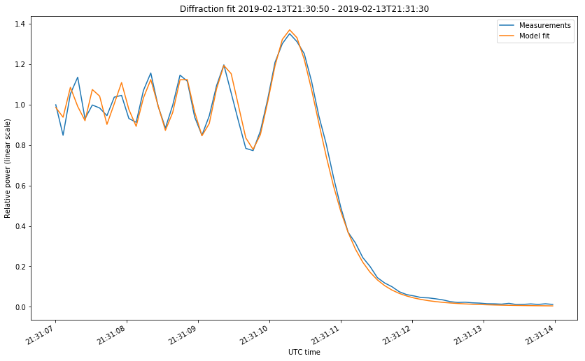
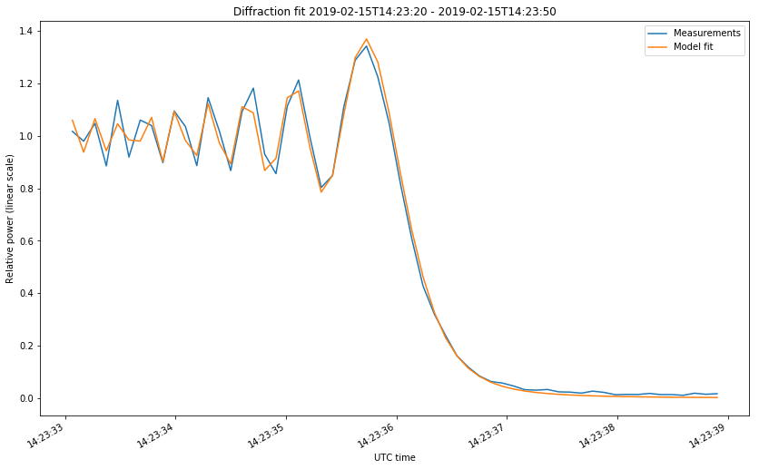
The first two figures correspond to the start of the occultations on February 4 and 13. The last two figures correspond to the start and end of the occultation on Februrary 15. The first figure looks somewhat different from the rest because the occultation was much slower. Take note at the time axis.
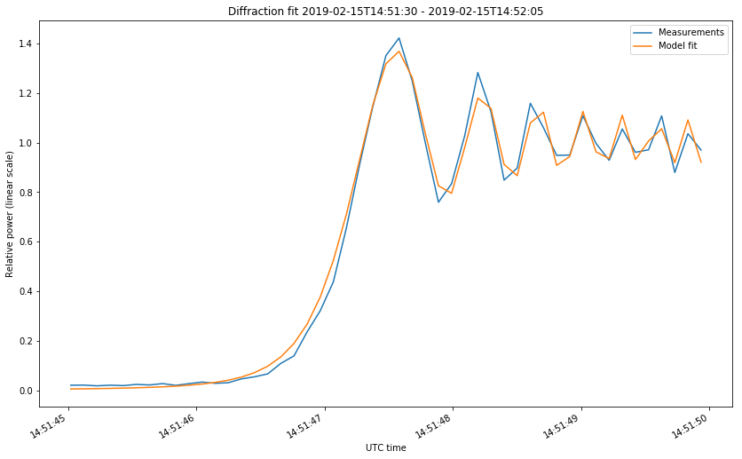
We can clearly see the diffraction fringes. Before dropping down to zero, the power of the received signal oscillates. The diffraction pattern that happens during a lunar occultation is explained in this document. There, the case of study is the occultation of a star by the Moon at optical wavelengths. In the derivation done in that document, it is implicitly assumed that the star is very far, so the wave arriving the Moon can be assumed to be a plane wave. This is not the case for DSLWP-B, which is much more near to the Moon. In this case, we need to consider a point source instead of a plane wave. The same kind of diffraction pattern is obtained in both cases, but the temporal frequency at which the diffraction fringes occur (the fringe rate) can be quite different, especially because the distance from DSLWP to the surface of the Moon is changing quickly.
The typical diffraction pattern is given by the Fresnel integral\[D(\nu) = \frac{1}{2}\left|\int_{-\infty}^\nu e^{i\pi s^2/2}\,ds\right|^2.\]A plot of this function can be seen in the figure below.
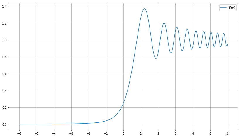
The variable \(\nu\), depends on the geometry of the diffraction, and is computed differently in the case of a plane wave or a point source. The point \(\nu=0\) represents the case of a grazing diffraction, which means that the line of sight path is tangent to the obstacle. The case \(\nu < 0\) corresponds to the situation when the direct line of sight is blocked, and \(\nu > 0\) corresponds to the situation when there is a direct line of sight path. As the obstacle gets away from the line of sight and \(\nu \to +\infty\), we have \(D(\nu) \to 1\), so we recover the power we would have if the obstacle wasn’t present.
Without discussing for now much about the geometry of the problem and how to compute \(\nu\) with respect to time \(t\), we just assume that it is reasonable to approximate \(\nu\) by its first order Taylor expansion about the instant \(t_0\) when the grazing diffraction happens:\[\nu \approx v(t-t_0).\]
The next step in the analysis is to fit a function of the form\[P_0D(v(t-t_0))\]to the observed data, where \(P_0\), \(v\), and \(t_0\) are unknown parameters representing the unobstructed signal power, the fringe rate, and the instant of grazing respectively.
To that end, we use a non-linear least squares fit. It is important to choose the initial values for the unknown parameters correctly to avoid falling in a local minimum. We do the following educated guesses. For \(t_0\) we take the instant when the power achieves its average value. To estimate \(v\) we try to locate the first local minimum and maximum of the diffraction fringes and compute \(v\) in terms of their temporal spacing. Finally, \(P_0\) is estimated as the mean value of the power after the first local minimum. The time interval over which the fit is performed is selected by hand. Also, averaging of the data is performed for the first occultation.
After taking these precautions, the fit is rather good, as shown in the figures below.
The fit gives us empirical values for \(t_0\) and \(v\). Let us compare those with the theoretical values obtained by using the tracking files from dslwp_dev as ephemeris and propagating the orbit in GMAT. This requires us to speak about how \(\nu\) is computed in terms of the geometry, for the case of a point source.
This is treated in this text very succinctly. It states that\[\nu = \pm2\sqrt{\frac{\Delta}{\lambda}},\]where \(\lambda\) is the wavelength and \(\Delta\) is the difference in distances between a certain “reflected” path and the direct line of sight path. The sign \(\pm\) is chosen according as to whether the direct line of path is blocked or not, as explained above.
In more detail, assume that our transmitter and receiver are at points \(A\) and \(B\) respectively. Consider the point \(R\) in the obstacle that is closest to the line segment joining \(A\) and \(B\). Then \[\Delta = \|A-R\| + \|R-B\| – \|A-B\|,\] where \(\|P-Q\|\) denotes the distance between the points \(P\) and \(Q\). Thus, \(\Delta\) is the extra distance traveled by a ray that goes from \(A\) to \(B\) reflecting off \(R\).
As an interesting fact, we have that the time derivative \(d\Delta/dt\) is equal to the difference in Dopplers between the direct signal and the Moonbounce signal (see the Appendix in this post). However, we are not really interested in \(d\Delta/dt\) but rather in the time derivative of \(\nu\), which involves \(\sqrt{\Delta}\), so it is not easy to relate the fringe rate and the Doppler directly.
In the case of the lunar occultation of DSLWP-B, we compute \(\Delta\) as follows. From GMAT we get the coordinates of the points \(A\) and \(B\) corresponding to DSLWP-B and Dwingeloo, and \(M\), which corresponds to the centre of the Moon. We compute the distance \(\delta\) between \(M\) and the line passing through \(A\) and \(B\) by computing \[l = \frac{\langle M – B, A – B\rangle}{\|A-B\|},\]the projection of the vector joining Dwingeloo and the Moon onto the unit line of sight vector pointing from Dwingeloo to DSLWP-B. Then\[\delta = \sqrt{|M-B|^2 – l^2}.\]We note that\[\Delta = |\delta – r|,\]where \(r\) is the lunar radius, and that the sign of \(\nu\) coincides with the sign of \(\delta – r\).
The instant of grazing diffraction is found by locating the time \(t_0\) for which \(\Delta = 0\). Then, the time derivative \(\frac{d\nu}{dt}(t_0)\) is evaluated numerically as a difference quotient.
For each of the four diffractions studied in this post, we obtain the following time differences in seconds between the instant of grazing \(t_0\) obtained from the fit to the measurements and the GMAT simulation:
[-116.05367306500001, 13.311127206, 31.371431057000002, 41.360679158]
We see that there are errors on the order tens of seconds. This can be explained by errors in the ephemeris. Indeed, it is difficult to estimate the mean anomaly of the orbit accurately, and it is the first parameter that becomes inaccurate with time, since orbital perturbations always build up in the mean anomaly. An offset in mean anomaly translates directly into a time offset in the instant of grazing. Determining accurately the instant of grazing is actually a good way to measure the mean anomaly precisely.
It is also interesting to observe the last two time differences, which correspond to the entry and exit of the same occultation on February 15. They have a difference of 10.01s, meaning that the duration of the occultation had such a difference between the observations and the GMAT prediction. This could also be explained by ephemeris errors, but the situation is not as simple as an offset in the mean anomaly.
The relative errors in the calculation of the fringe rate \(\frac{d\nu}{dt}(t_0)\) between the observations and the GMAT prediction are shown below in parts per one:
[0.012628611461853678, -0.14849525967852584, 0.03838583537440288, 0.021923209485447237]
We observe errors between 1% and 15%. This means that our model for the geometry of the diffraction explains the observations very well.
The grazing instants determined from the observations are
2019-02-04T10:06:58.345423935
2019-02-13T21:31:11.257607206
2019-02-15T14:23:36.420400057
2019-02-15T14:51:46.844356158
The fringe rates, in units of 1/s determined from the observations are
[-0.1682628343896966, -1.2532957532402556, -1.7370407299575834 1.6895344971498276]
The computations and plots shown in this post have been done in this Jupyter notebook.
Fascinating – reminds me of an old experiment “USING SHADOWED STARLIGHT AS A YARDSTICK” { https://archive.org/stream/TheAmateurScientist/Stong-TheAmateurScientist_djvu.txt } describing diffraction of starlight by the moon