Last week I did an experiment where I transmitted WSPR on a fixed frequency for several days and studied the distribution of the frequency reports I got in the WSPR Database. This can be used to study the frequency accuracy of the reporters’ receivers.
I was surprised to find that the distribution of reports was skewed. It was more likely for the reference of a reporter to be low in frequency than to be high in frequency. The experiment was done in the 40m band. Now I have repeated the same experiment in the 20m band, obtaining similar results.
The details of the experiment are contained in the previous post. This time I have been transmitting on 14097100Hz, and after measuring against my GPSDO I have determined that my real transmit frequency was 14097098.43Hz. The test has run over the course of 6 days, collecting a total of 3643 reports coming from 146 different reporters. Below you can see the distribution of the frequency error of the reporters.
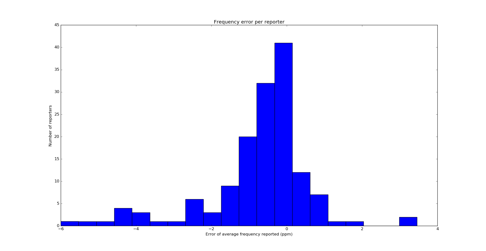
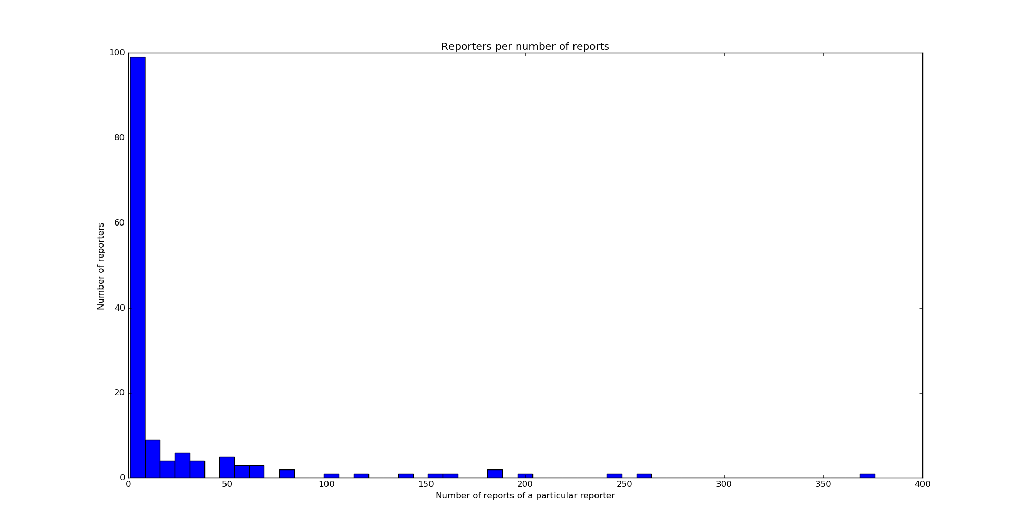
The distribution is similar to the one obtained on 40m, but it is not quite the same. Nevertheless, both distributions are clearly skewed to the left. Below you can see the histograms showing the reporters per number of reports. We see that most reporters have only given 10 reports or less.

When I tweeted about this bias in frequency, several people presented theories to try to explain the bias. F4DAV suggested that this could be an artefact of the WSPR decoder. However, I have contacted Joe Taylor to check if the software could play any role, and he doesn’t think so. He remarks that he has done tests with K9AN using a GPS-locked system and a well calibrated transceiver and they obtain reports which are accurate to 1Hz (note that 1Hz is 0.1ppm in 40m, and here we are seeing much larger biases).
Miguel Ángel EA4EOZ remarked that it is not so easy to derive the frequency error of the reference of a receiver given the frequency error in the WSPR report (which is measured at the audio output by the WSPR software). He said that this depends on the receiver architecture and how many stages it has in the case of a superhet receiver. This left me wondering for a while, as it occurred to me that according as to whether the first LO was below or above the RF frequency you would see the frequency error go in a different direction.
A moment’s thought shows that this is not the case: the architecture of the receiver doesn’t matter at all. At the audio output you will get an error in frequency which equals the relative error of the frequency reference of the receiver times the RF frequency of the signal. It doesn’t matter if the receiver is a superhet having several stages, a direct conversion zero-IF SDR or a direct sampling DDC SDR (in the case where the receiver has frequencies derived from different crystal oscillators you should replace the concept of “frequency reference” by a suitable weighted average of all the crystal oscillators).
My favourite way to see this is that the frequency reference of a receiver is used to measure time. It’s the receiver’s clock. It doesn’t matter how it’s used to bring the RF signal down to AF. If the receiver’s clock is running slow, the RF will appear higher in frequency and vice versa.
Another way to see it is to think that each stage in a superhet receiver performs a frequency conversion where the RF frequency \(f^{\text{RF}} = f^{\text{IF}}_0\) is transformed into the first IF, \(f^{\text{IF}}_1\), by \(f^{\text{IF}}_j = \pm f^{IF}_{j-1} \pm f^{\text{LO}}_j\), with the condition that \(f^{\text{IF}}_j \geq 0\), so in particular both signs cannot be \(-\) simultaneously. After several frequency conversions we arrive at the AF, \(f^{\text{AF}} = f^{\text{IF}}_n\) and we can groups all the \(f^{\text{LO}}_j\) terms as \(f^{\text{LO}} = -(\pm f^{\text{LO}}_1 \pm \cdots \pm f^{\text{LO}}_k)\). Hence, \(f^{\text{AF}} = \pm f^{\text{RF}} – f^{\text{LO}}\). Now, the fact that the frequency conversion from RF to AF is sideband preserving (i.e., the mode is USB), means that \(f^{\text{RF}}\) should have the sign \(+\). Note that this forces \(0 < f^{\text{LO}} < f^{\text{RF}}\). If the receiver uses only a single crystal, then each of the frequencies \(f^{\text{LO}}_j\) is a constant multiple of the frequency of the crystal, so the same is true of \(f^{\text{LO}}\). If the receiver uses several crystals, then \(f^{\text{LO}}\) is a linear combination of the frequencies of all the crystals. Note that the coefficients may have positive and negative signs, which can get interesting. In the usual case the crystal whose frequency error dominates the error in \(f^{\text{LO}}\) will have a positive coefficient in the linear combination, but there can be pathological cases. The same kind of reasoning done here applies for a direct conversion zero-IF receiver or a DDC.
Miguel Ángel EA4EOZ has also made a key remark: crystals only go down in frequency when they age. This is almost true. As this image shows, there is an increase in frequency due to stress relief and a decrease in frequency due to mass transfer. In the long run, the decreasing effect wins out. This seems a convincing cause that explains the bias I am seeing in the frequency distribution. Amateur transceivers are calibrated on fabrication but eventually their crystals age and go down in frequency, and most hams don’t bother to calibrate the transceiver frequently.
One comment