This post is a continuation of my series about LTE signal analysis. In the previous post I showed how to decode the PHICH. Now we will decode two other downlink channels, the PBCH (physical broadcast channel) and the PDDCH (physical downlink control channel).
The PBCH is used to transmit the MIB (master information block). This is a small data packet that all the UEs must decode after detecting a cell using the synchronization signals. The MIB contains essential information for the usage of the cell, such as the cell bandwidth and PHICH configuration. The PDDCH contains control information, such as uplink grants and the scheduling of the PDSCH (physical downlink shared channel).
The PBCH and PDDCH use the same kind of channel coding: a tail-biting k=7, r=1/3 convolutional code with a circular buffer for rate matching that performs puncturing and repetition coding as needed to obtain the required codeword size. The remaining aspects of the PBCH and PDDCH are quite different, so they will be treated separately.
As usual, we will be using a short IQ recording from my local cell site. The link to the recording is given at the end of the post.
PBCH transmissions
We have already looked at the demodulation of the PBCH in the post about reference signals and transmit diversity. The PBCH is transmitted in the first 4 symbols of slot 1 in each radio frame. A complete PBCH codeword (which carries an MIB message) takes 4 radio frames (40 ms) to be transmitted. The PBCH only uses the 6 central resource blocks, since those are present even in the narrowest LTE cells, which have a bandwidth of 1.4 MHz. Moreover, since by the time that a UE tries to receive the PBCH it does not know how many antenna ports are used for the CRS (cell-specific reference signals), the PBCH avoids all the resource elements that would be used by a 4-port CRS.
The PBCH can use either one antenna port (port 0) or transmit diversity on 2 ports (ports 0, 1) or 4 ports (ports 0, 1, 2, 3). At first the UE doesn’t know the configuration in use, so it tries to detect it blindly by trying the different equalizations. The correct configuration is confirmed when the UE decodes the MIB. In this recording we already know that the PBCH uses transmit diversity on 2 ports.
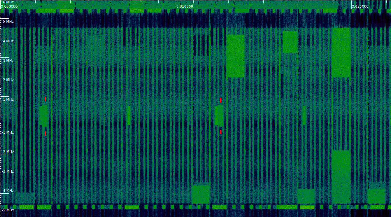
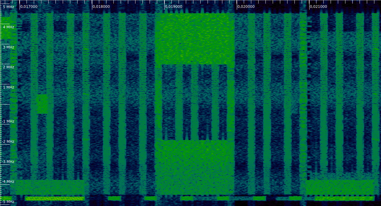
The figure below shows the waterfall at the beginning of the recording, with the first two PBCH trasmissions marked with red ticks. We can see the synchronization signals, which are slightly narrower than the PBCH, being transmitted every 5 ms. The PBCH comes immediately after the synchronization signals every other time.
PBCH channel coding
Each PBCH transmission consists of 240 resource elements, as there are 8 resource elements per resource block allocated to the PBCH in each of the first 2 symbols (due to the potential presence of the CRS) and 12 resource elements per resource block in each of the last 2 symbols. The modulation is QPSK, so there are 480 bits per transmission. Since an MIB transmission takes up 4 consecutive PBCH transmissions, the MIB codeword has 1920 bits.
The MIB itself has 24 bits, plus a 16 bit CRC. These 40 bits are encoded as a 1920 bit codeword so that the MIB can be decoded even with very bad signal quality. An UE that receives the PBCH with good SNR is able to decode the MIB from just the 480 bits of a single PBCH transmission, speeding up the decoding process.
The channel coding for the PBCH is described in Section 5.3.1 of 3GPP TS 36.212. First, the CRC-16 of the 24-bit MIB message is computed. The CRC algorithm is CRC16_CCITT_ZERO in this online calculator. The CRC is masked (XORed) with a bit pattern that indicates the number of antenna ports used by the eNB. This masking technique is a funny idea used by LTE to transmit slightly more information “for free” at the cost of making the CRC-16 slightly weaker. The CRC is masked with 0x0000 for 1 antenna port, with 0xffff for 2 antenna ports, and with 0x5555 for 4 antenna ports. A UE will try to check the CRC using the 3 possible masks, and if it gets a successful check, it will know the number of antenna ports and that the 24 bit MIB is error free.
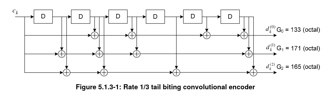
The 40 bits obtained by the concatenation of the 24 bit MIB and the CRC-16 are sent into the convolutional encoder. This is a k=7, r=1/3 encoder that is used in a tail-biting manner, which means that the shift register is initialized with the last bits of the message, so that the shift register contents at the beginning and end of the encoding match.
The encoder is shown in the figure below. It produces 3 vectors of 40 bits when used with the MIB.
The three vectors produced by the convolutional encoder are sent into a rate matching algorithm. This gives a way of decoupling the input (information block) size from the output (codeword) size by performing puncturing and repetition as needed. It also performs interleaving to add robustness against burst errors.
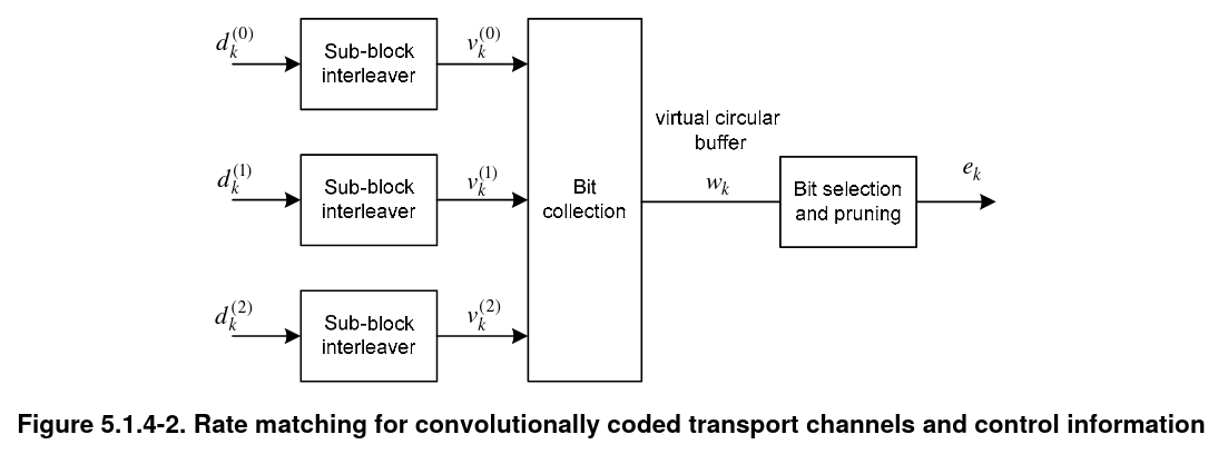
The sub-block interleaver step is performed in the same way and separately for each of the 40 bit vectors. First, the vector is written by rows into a matrix with 32 columns and \(\lceil D/32 \rceil\) rows, where \(D\) denotes the length of the input vector. In the case of the MIB, \(D = 40\), so 2 rows are needed, but all these steps are defined for generic input and output sizes. Whenever \(D\) is not divisible by 32, <NULL> elements are added in the last entries of the matrix (here <NULL> denotes a symbolic element that will be punctured later). The 32 columns of the matrix are permuted following a fixed permutation, and then data is read by columns, including <NULL> elements. This gives the output of the sub-block interleaver.
The bit collection step simply concatenates the 3 outputs produced by the sub-block interleavers. The bit selection and pruning step works as follows. We imagine the output of the previous step as a circular buffer. We start at the beginning of this buffer, and iterate over the elements of the buffer, copying bits to the output and skipping over any <NULL> elements. We stop when we have obtained exactly the codeword size we need. Depending on the required coding rate, it may be necessary to do a fraction of a lap around the circular buffer or several laps.
For the PBCH we need to obtain 1920 bits from a buffer that has 120 non-<NULL> elements, so exactly 16 laps around the buffer are needed. This means that for the particular case of the PBCH, we can see the rate matching as a simple 16x repetition coding. The 40 bit MIB is encoded into 120 bits by an r=1/3 convolutional code. These 120 bits are repeated 4 times to fill the 480 bits in a PBCH transmission, and the same data is repeated in 4 consecutive PBCH transmissions.
The 1920 bit codeword obtained from the rate matching algorithm is scrambled with a 1920 bit pseudorandom sequence that is obtained from the PCI (physical cell ID) with the usual LTE pseudorandom sequence generator. This implies that the 4 consecutive PBCH transmissions that compose an MIB do not carry the same symbols, as the codeword bits are scrambled differently in each of the transmissions.
Decoding the MIB
As mentioned above, the MIB is transmitted every 40 ms, and uses 4 consecutive PBCH transmissions. The synchronization signals give to the UE the cell time modulo 10 ms, so after synchronization it is able to demodulate the PBCH. However, the UE doesn’t know yet the cell time modulo 40 ms, so to decode the MIB it needs a trial and error process. Often, this is done with a sliding window that contains the last 4 PBCH transmissions. One out of every 4 transmissions, the window will be aligned to the 40 ms boundaries correctly and the UE will be able to decode the MIB. The successful decode of the MIB confirms the cell time modulo 40 ms.
If the SNR is good, a UE can attempt to decode the MIB from a single PBCH transmission, to avoid to wait 40 ms to gather 4 transmissions. In this case, the UE needs to try all the 4 possible options regarding the time alignment of the PBCH transmission in order to de-scramble the single PBCH transmission.
In our case, in order to validate the implementation of each of the decoding operations as independently as possible, we do the following. First, we form a sliding window of 4 PBCH transmissions, obtain the 1920 bit vectors from each window, and de-scramble each of these vectors.
Now we run the rate matching algorithm in reverse, mapping each of these 1920 bits to the corresponding convolutional codeword bit \(d^{(j)}_k\). For each of these \(d^{(j)}_k\)’s we get a set of 16 bits (due to the repetition encoding). We compute the variance of each of these groups, and then compute the average of these variances over the 120 bits \(d^{(j)}_k\). We call this the “score”.
When the sliding window is correctly aligned to the 40 ms boundaries, the de-scrambling will be correct and in each group of 16 repetitions we will find 16 copies of the same bit. Therefore, the score will be low. Conversely, when the alignment of the sliding window is not correct, the de-scrambling will be wrong and each of the 16 bit groups will have 16 random-like bits. Therefore, the score will be high. By looking at the score, we can figure out the correct 40 ms boundaries.
The figure below shows a plot of the score in terms of the first frame that is put into the 4 frame window. We see that the score is low when we start with frames 3, 7, 11, etc.
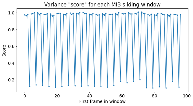
From the plot of the score we know that the first PBCH transmission in the recording corresponds to the second of the 4 transmissions that comprise an MIB. For simplicity, we discard the first 3 PBCH transmissions to align ourselves to the start of the MIB, and collect the remaining PBCH transmissions in groups of 4.
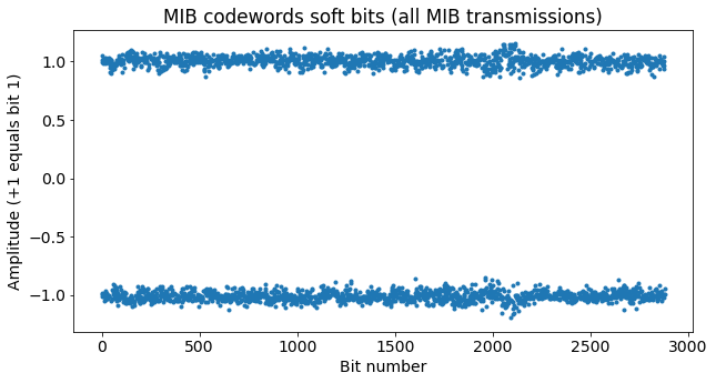
We take the 1920 bits corresponding to each MIB (already de-scrambled), and again we reverse the action of the rate matching algorithm to group these in 120 groups of 16 bits each. We compute the average of each group, thus obtaining a good estimate for the bits of the convolutional codewords.
The concatenation of the convolutional codeword bits for all the MIB transmissions in the recording is shown in the next figure. We see that the SNR is very good and there is no chance for bit errors in our case. Indeed, we could have attempted to decode the MIB from a single PBCH transmission.
To decode the convolutional code, I have done a simple Python implementation of the Viterbi decoder. I have followed Sarah Johnson’s book Iterative Error Correction (see Algorithm 4.3 in the book).
The convolutional code used by LTE is tail-biting, so this needs to be taken into account in the Viterbi decoder. There are several possible ways to address this. One way is to start the trellis at any state (for instance, the state where all the bits in the encoder shift register are zero), process the complete codeword, and then continue past the end of the codeword, repeating again the first bits. At some point we can trace back the path of lower cost, recovering first the beginning of the message from this “second lap”, and then the end of the message from the end of the “first lap”.
Another approach is to do a run of the Viterbi decoder for each of the possible state values, enforcing that the initial and final state of the trellis should equal each of the values. The decoder output corresponds to the path of lower cost overall. This has the disadvantage that it is much more costly, since we need to run the Viterbi decoder \(2^{k-1}\) times, where \(k\) is the constraint length (\(k = 7\) for LTE). On the other hand, it gives the best results (it gives the maximum likelihood decode), and is simple to implement. Therefore, I have followed this approach.
To check that the Viterbi decoder is working correctly, we can encode again one of the messages produced by the Viterbi decoder and check that it matches the original codeword.
After running the Viterbi decoder for each of the MIB transmissions, we obtain 24 MIBs of 40 bits each. These are shown below as a raster map, with each MIB being represented as a row.
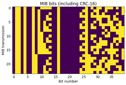
In the raster map we can see that there is a binary counter in bits 6 through 13. This field is the System Frame Number (SFN), or actually the 8 most significant bits of the 10-bit SFN since the 2 least significant bits are given implicitly by the alignment of the MIB (the MIB transmissions start on the subframes in which these 2 least significant bits are zero). The 16 rightmost bits in the raster map correspond to the CRC, which explains their variability.
As mentioned above, the CRC is masked with a pattern that indicates the number of antenna ports used for the CRS. As we know that the this cell uses 2 ports, we can mask the CRC with the corresponding pattern, 0xffff, and check that all the CRCs are correct.
The structure of the MIB is defined in ASN.1 in TS 36.331. The relevant ASN.1 code is given below.
MasterInformationBlock ::= SEQUENCE {
  dl-Bandwidth ENUMERATED {n6, n15, n25, n50, n75, n100},
  phich-Config PHICH-Config,
  systemFrameNumber BIT STRING (SIZE (8)),
  schedulingInfoSIB1-BR-r13 INTEGER (0..31),
  systemInfoUnchanged-BR-r15 BOOLEAN,
  spare BIT STRING (SIZE (4))
}

PHICH-Config ::= SEQUENCE {
  phich-Duration ENUMERATED {normal, extended},
  phich-Resource ENUMERATED {oneSixth, half, one, two}
}
I have used the Python package asn1tools to compile this ASN.1 code and parse the MIBs we have received. The field values of the first MIB are shown below.
{'dl-Bandwidth': 'n50',
 'phich-Config': {'phich-Duration': 'normal', 'phich-Resource': 'one'},
 'systemFrameNumber': (b'O', 8),
 'schedulingInfoSIB1-BR-r13': 4,
 'systemInfoUnchanged-BR-r15': False,
 'spare': (b'\x00', 4)}
The cell bandwidth is 50 resource blocks, which corresponds to 10 MHz. As we already found by looking at the signal in the previous post, the PHICH uses normal duration and \(N_g = 1\) (the \(N_g\) parameter is used to define how many REGs are allocated to the PHICH). The 8 MSBs of the SFN count from 79 to 102.
PDCCH
The PDCCH, or physical downlink control channel, is used to transmit all the control information that is not carried by any of the other channels (PBCH, PCFICH, PHICH). This control information consists of uplink grants and PDSCH scheduling. The messages sent by the PDCCH are called DCIs (downlink control indicator). There are many different types of DCI formats, as the format to use depends on the type of transmission it refers to (whether it uses MIMO, etc.).
The PDCCH is transmitted in the REGs of the control region which are not allocated to the PCFICH and the PHICH. Recall that a REG is a set of 4 resource elements which are adjacent in frequency if we ignore the resource elements used by the CRS. The control region is the first 1, 2 or 3 symbols of the subframe. The size of the control region (i.e., 1, 2, or 3 symbols) is given by the CFI (control format indicator) carried in the PCFICH of each subframe.
In each subframe, several DCIs can be transmitted at a time. Depending on the size of the control region and the number and coded size of the DCIs to send, the PDCCH may use all its REGs or leave some of them empty. This can be seen easily in the waterfall.
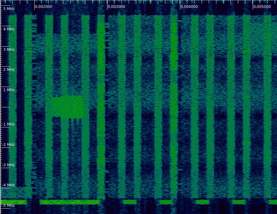
The first example of a waterfall shows two PDCCH tranmissions with CFI=1 that occupy all the REGs allocated to the PDCCH (near 0.003 and 0.004 seconds). Note that the 4 subcarrier regions allocated to the PHICH are left empty (see the previous post), although there is a PHICH transmission active in one of these. In the first and last subframe of this waterfall we can see that the PDCCH is not transmitting anything.
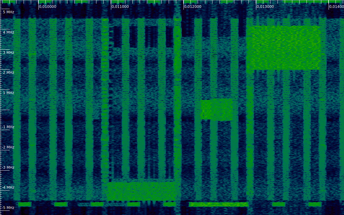
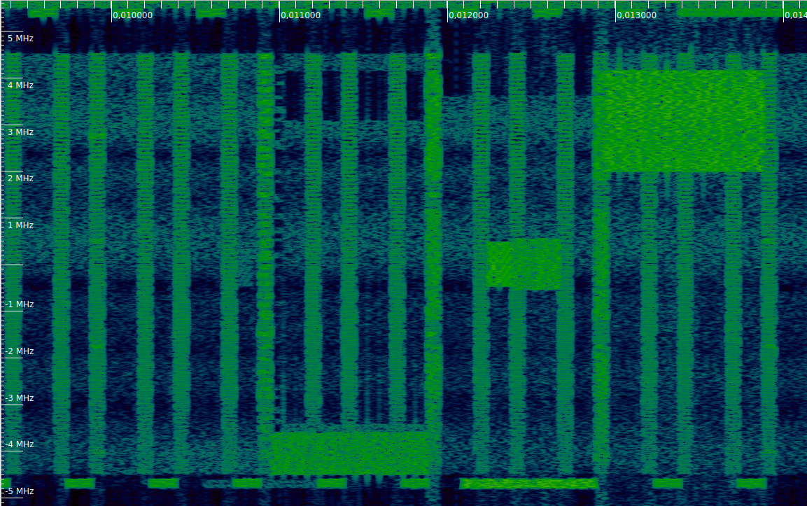
In the next example, we can see that in the second subframe (near 0.011 seconds) the PDCCH only uses about half of the REGs, leaving the remaining REGs free. Compare with the next two subframes, where all the REGs of the PDCCH are active.
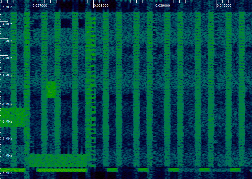
The last example shows a PDCCH with CFI=2 (near 0.038 seconds). The transmission is distributed over all the set of REGs allocated to the PDCCH, as we will see below. Since the total allocation is now much larger, there are many free REGs that remain inactive. There are no examples of CFI=3 in this recording.
PDCCH mapping to resource elements
The PDCCH uses the concept of CCEs (control channel elements) to define how the resource elements are allocated. A CCE is a set of 9 REGs. Therefore, a CCE contains 36 resource elements, and since the PDCCH uses QPSK, it carries 72 bits.
The DCIs to transmit must be encoded (as described below) to occupy either 1, 2, 4 or 8 CCEs (72, 144, 288, or 576 bits). The number of CCEs occupied by a DCI codeword is called aggregation level. The 4 possible aggregation levels define the PDCCH formats 0, 1, 2, 3 (this is just another name for the possible choices of aggregation levels).
The CCEs that are available in the control region of a subframe (which depends on the number of REGs in that region, and ultimately on the CFI, as well as on the number of REGs allocated to the PHICH) are numbered as 0, 1, etc. A DCI should be mapped to adjacent CCEs according to this numbering, with the additional restriction that it should start on a CCE whose index is divisible by the aggregation level (i.e., a DCI with an aggregation level of 8 can only start at CCEs 0, 8, 16, etc.). If necessary. <NIL> symbols are inserted to occupy all the available CCEs and to align the DCIs according to their aggregation level. Likewise, when the total number of REGs in the control region is not a multiple of 9, the last REGs are also filled with <NIL> symbols. The <NIL> symbols are transmitted as zeros, and cause the empty resource elements that we have seen in the waterfall.
The resulting vector of bits corresponding to all the REGs allocated to the PDCCH (including <NIL> symbols) is scrambled with a pseudorandom sequence that depends on the PCI and the subframe number.
The interesting aspect is that the PDCCH REGs are not mapped in order to resource elements. Instead, they are permuted before being mapped. The permutation is defined in the same way as in the channel coding interleaver (see the description of the PBCH channel coding above). In this case it acts on REGs (the 4 resource elements in each REG are permuted together as a whole), and <NULL> elements inserted by the interleaver are removed. After performing this permutation (which only depends on the total number of REGs), the resulting REGs are shifted cyclically using the PCI in order to make the placement of the REGs different for each cell.
Finally, the permuted and shifted REGs are mapped to the time-frequency grid in the following way. REGs are chosen in increasing order according to the frequency of the lowest resource element in the REG, and in case of ties according to the symbol number (i.e., lexicographic order in frequency and time). Note that only REGs that are not allocated to the PCFICH and PHICH are considered for this mapping.
These permutation operations, as well as the lexicographic order in frequency and time are what cause the sparse patterns in the control region that we have seen in the waterfall whenever the PDCCH is not completely full.
PDCCH channel coding
The channel coding for each DCI is defined in the same way as for the PBCH. First there is a tail-biting convolutional encoder, followed by interleaving of each codeword, and finally a rate matching using a circular buffer to obtain the desired codeword size.
The codeword size is restricted to 72, 144, 288 or 576 bits depending on the aggregation level used for this DCI. The input size depends on the DCI format, and also on the cell bandwidth and whether the cell is FDD or TDD. The table below shows that there are many different DCI formats with different sizes.

As in the case of the MIB, the DCIs include a 16-bit CRC. The CRC is masked with the so called RNTI (radio network temporal identifier), which is a 16-bit number used to define to which UE or UEs the DCI is addressed. Each UE that is connected to the cell will be assigned a different C-RNTI (cell RNTI). DCIs can be addressed to a UE individually by masking the CRC with its C-RNTI. There are also special RNTIs which address multiple UEs, such as the P-RNTI (paging RNTI) 0xfffe and the SI-RNTI (system information RNTI) 0xffff. Each UE will only attempt to unmask the CRC with each of its assigned RNTIs, thus ignoring DCIs addressed to other UEs.
Additionally, the CRC of some DCI formats can also be scrambled with a pattern for closed-loop selection of the UE transmit antenna port. To indicate port 0, the pattern 0x0000 is used, while the pattern 0x0001 corresponds to port 1.
Decoding the PDCCH
The first step to prepare the decodification of the PDCCH is to compute the permutations of the REGs. We need to be able to map from the resource elements obtained in the OFDM demodulation to the REGs in the order in which they conform the CCEs. There is a different mapping for each CFI value, since the total number of available REGs depends on the CFI. Additionally, we also need to know the number of REGs allocated to the PHICH (we computed this in the previous post).
To validate that the permutations of the REGs are being done correctly, it is helpful to choose subframes for which the PDCCH is not full (i.e., those that look sparse in the waterfall). After undoing the REG permutation we should see that the active REGs are adjacent, match the four possible aggregation levels, and are correctly aligned.
For this particular cell, with CFI=1 the PDCCH has 75 REGs, which gives 8 CCEs (plus 3 extra REGs which are always unused), while with CFI=2 the PDCCH has 225 REGs, which gives exactly 25 REGs.
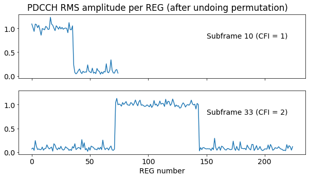
The figure below shows the RMS amplitude of each REG after undoing the permutation for two subframes in which the PDCCH is not full. In the subframe with CFI = 1 we can see that the first 4 CCEs are in use. We will later see that this corresponds to a single DCI with aggregation level 4. In the subframe with CFI = 2 we see that 8 CCEs are in use. These start at CCE number 8, so the alignment is correct. They also correspond to a single DCI.
A UE decodes the PDCCH by a “blind decoding” procedure. The UE monitors a certain set of CCEs (potentially not all of them, to reduce the amount of calculations to be done), attempting to decode using all the possible combinations of aggregation levels and DCI sizes in these CCEs. It tries to mask the CRC of the DCIs with each of its RNTIs (typically, a C-RNTI, and the P-RNTI and SI-RNTI), and processes as valid all the DCIs for which the CRC check is successful. In this way the UE obtains all the DCIs addressed to it without any prior knowledge of their sizes, aggregation levels and locations. It also discards all the DCIs not addressed to it, and any combination of parameters which doesn’t match one of the DCIs that were transmitted.
For a monitoring application such as the analysis of the recording we are doing here, this blind decoding approach is not very useful, because we do not know the set of RNTIs that we should see. Potentially we could monitor the P-RNTI and SI-RNTI in a blind decoding approach, but we don’t know the C-RNTIs of the connected UEs. Therefore, here we use some heuristics to try to detect by hand the parameters of the DCIs. The main heuristic is that since this cell is not very busy, often at most one DCI is transmitted in the PDCCH. Therefore, by looking at the RMS amplitude we can directly determine which CCEs are occupied by the DCI. Things get more complicated when there are two or more DCIs allocated to adjacent CCEs, since we need to choose how to divide the CCEs.
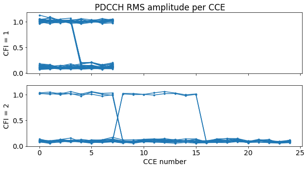
To determine which groups of CCEs are in use, first we plot the RMS amplitude of each CCE for the first 50 subframes in the recording. We do separate plots for CFI = 1 and CFI = 2, and plot all the subframes on top of each other. We can clearly see that for CFI = 1 the CCEs are allocated with a granularity of 4. In fact, either no CCEs are in use, or the first 4 CCEs are in use, or all the CCEs are in use. For CFI = 2 the CCEs are allocated with a granularity of 8. Either the first 8 CCEs, or the next 8 CCEs are used.
This is what happens for the first 50 subframes of the recording. If we study all the recording, then some additional patterns appear. However, we will only study the first 50 subframes in this post, since the DCIs are selected manually.
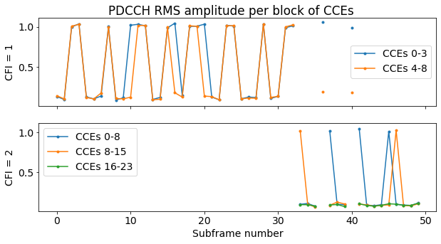
Now we can group the CCEs according to their use following the plot above and plot the RMS amplitude of each block of CCEs versus the subframe number. Again, we do this separately for CFI = 1 and CFI = 2. This plot shows which CCEs are used for each subframe.
Before proceeding further we also need to de-scramble the received PDCCH symbols. This is straightforward to do, since it doesn’t require knowledge of what CCEs are in use or how the DCIs are encoded. It is only necessary to know the CFI of each subframe and to undo the permutation of the REGs correctly. After this, the scrambling sequence can be generated and applied to the symbols.
Now let us take subframe 10 as an example to test the rest of the decoding procedure. We have seen above that in this subframe CCEs 0-3 are in use. As we will see, there is a single DCI occupying these 4 CCEs. We can plot the bits corresponding to these CCEs. These are already de-scrambled. There are 288 bits, as expected for aggregation level 4.
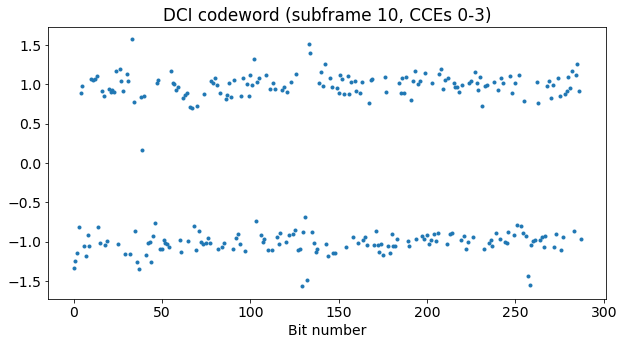
To deduce the size of this DCI, we use a variation of the idea that we used to detect the MIB alignment. For each DCI size candidate, we run the rate matching algorithm in reverse to group the symbols according to the convolutional codewords bit to which they correspond. Then, in each of the groups we compute the maximum distance between pairs of bits in the group, and define the score as the overall maximum of these distances. The idea is that, for the correct size, all the groups will contain copies of the same bit, and so the distances will be small, while for a wrong size there will be groups containing different bits with opposite values, causing a large distance.
The plot of the score is shown below. We see that there is a significant drop at DCI size 43. This size indeed matches the sizes for DCI formats 0, 1A, 3 and 3A, according to the table above. There is also another drop at 86, because this is a multiple of the correct DCI size, so the groups that are formed when reversing the rate matching are subsets of the groups for size 43. When the size candidate is large enough, the score drops to 0, as the coding rate is then higher than 1/3, and so the rate matching does not repeat any bits.

As for the MIB, we now run in reverse the rate matching for the correct DCI size and compute the average of each group of bits. We obtain the convolutional codewords, which amount to 129 bits in total (43 times 3). As in the case of the MIB, the SNR is quite good and there are no bit errors.
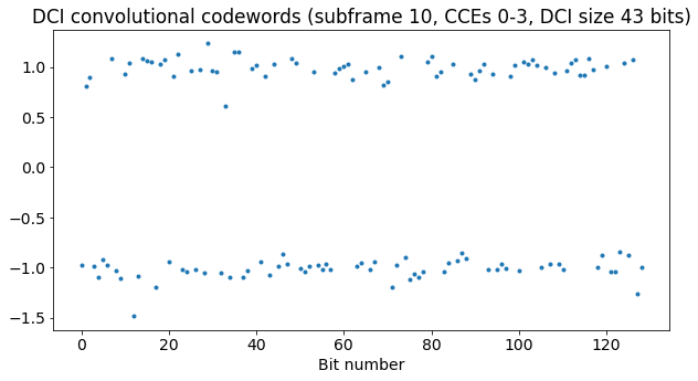
Now we run the tail-biting Viterbi decoder on these codewords to obtain the 43 bit DCI. To find the mask of the CRC, we simply compute the CRC of the DCI (using the first 27 bits of the DCI) and calculate its XOR against the CRC in the last 16 bits of the DCI. The result is 0xfffe, which is the P-RNTI. Thus, we are confident that we have decoded the DCI correctly.
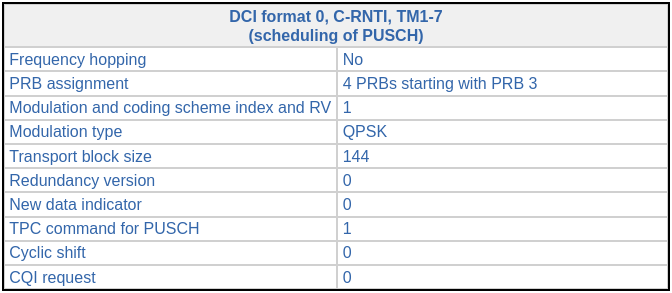
The contents of each DCI format are given in Section 5.3.3.1 of TS 36.212. However, this section is very detailed, as there are many DCI formats and variations. A simpler alternative to get the contents of a DCI is an LTE DCI decoder webpage where we can enter the DCI in hex and obtain the values of its fields. This DCI is 86408040, and has a length of 27 bits (the webpage doesn’t need the CRC). Entering these values, as well as the cell parameters (FDD, 10 MHz, 2 antenna ports), we obtain some possible interpretations for this DCI. The only one that matches the P-RNTI is the following.
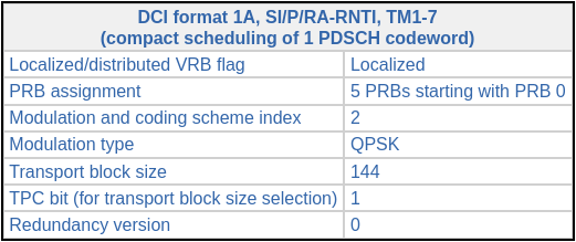
If we look at the area of the waterfall where this DCI is transmitted, we see that the information in the DCI is correct. In the figure below we note that there is a PDSCH transmission occupying the 5 lower resource blocks of the cell. This is the transmission described by the DCI given above, so now we know that this PDSCH transmission contains paging data.
Now we look manually at all the PDCCH in the first 50 subframes or so of the recording. Besides DCIs of size 43, we also see DCIs of size 59. The plot below gives the scores for a few selected DCI codewords with different CFIs and sizes. DCI size 59 corresponds to DCI format 2.

By giving a manually generated list of subframes, CCE ranges, and DCI sizes, the decoding can proceed. The results are shown below. We see that besides the P-RNTI and SI-RNTI, there are two C-RNTIs present: 0xc33c, and 0xced8. The decoded DCIs in hex can be pasted directly on the decodder webpage. Subframe 50 is of special interest because it is the only one of these in which several DCIs are transmitted.
Subframe index 2: CFI 1, CCEs 0-7, 43 bit DCI
CRC-16 mask 0xc33c
DCI (hex, without CRC) 04c84800

Subframe index 3: CFI 1, CCEs 0-7, 43 bit DCI
CRC-16 mask 0xc33c
DCI (hex, without CRC) 03384800

Subframe index 7: CFI 1, CCEs 0-7, 43 bit DCI
CRC-16 mask 0xc33c
DCI (hex, without CRC) 04d02800

Subframe index 10: CFI 1, CCEs 0-3, 43 bit DCI
CRC-16 mask 0xfffe
DCI (hex, without CRC) 86408040

Subframe index 11: CFI 1, CCEs 0-7, 43 bit DCI
CRC-16 mask 0xc33c
DCI (hex, without CRC) 03487000

Subframe index 12: CFI 1, CCEs 0-7, 59 bit DCI
CRC-16 mask 0xc33c
DCI (hex, without CRC) 00079e080160

Subframe index 15: CFI 1, CCEs 0-7, 43 bit DCI
CRC-16 mask 0xc33c
DCI (hex, without CRC) 04d00800

Subframe index 16: CFI 1, CCEs 0-3, 43 bit DCI
CRC-16 mask 0xffff
DCI (hex, without CRC) 84b0c240

Subframe index 18: CFI 1, CCEs 0-7, 59 bit DCI
CRC-16 mask 0xced8
DCI (hex, without CRC) 7c07ce101000

Subframe index 19: CFI 1, CCEs 0-7, 43 bit DCI
CRC-16 mask 0xc33c
DCI (hex, without CRC) 01bf6880

Subframe index 20: CFI 1, CCEs 0-3, 43 bit DCI
CRC-16 mask 0xfffe
DCI (hex, without CRC) 84b0c000

Subframe index 23: CFI 1, CCEs 0-7, 43 bit DCI
CRC-16 mask 0xc33c
DCI (hex, without CRC) 04d0a800

Subframe index 24: CFI 1, CCEs 0-7, 43 bit DCI
CRC-16 mask 0xc33c
DCI (hex, without CRC) 01b8a800

Subframe index 28: CFI 1, CCEs 0-7, 43 bit DCI
CRC-16 mask 0xc33c
DCI (hex, without CRC) 04c81000

Subframe index 31: CFI 1, CCEs 0-7, 59 bit DCI
CRC-16 mask 0xc33c
DCI (hex, without CRC) 00079e0c0160

Subframe index 32: CFI 1, CCEs 0-7, 59 bit DCI
CRC-16 mask 0xced8
DCI (hex, without CRC) 7007ceeb0160

Subframe index 33: CFI 2, CCEs 8-15, 43 bit DCI
CRC-16 mask 0xc33c
DCI (hex, without CRC) 01b8a800

Subframe index 36: CFI 1, CCEs 0-3, 43 bit DCI
CRC-16 mask 0xffff
DCI (hex, without CRC) 84b0c340

Subframe index 37: CFI 2, CCEs 0-7, 43 bit DCI
CRC-16 mask 0xc33c
DCI (hex, without CRC) 04d82800

Subframe index 40: CFI 1, CCEs 0-3, 43 bit DCI
CRC-16 mask 0xfffe
DCI (hex, without CRC) 83200040

Subframe index 41: CFI 2, CCEs 0-7, 43 bit DCI
CRC-16 mask 0xc33c
DCI (hex, without CRC) 04d80800

Subframe index 45: CFI 2, CCEs 0-7, 43 bit DCI
CRC-16 mask 0xc33c
DCI (hex, without CRC) 04d00800

Subframe index 46: CFI 2, CCEs 8-15, 43 bit DCI
CRC-16 mask 0xc33c
DCI (hex, without CRC) 01b88800

Subframe index 50: CFI 1, CCEs 0-3, 43 bit DCI
CRC-16 mask 0xfffe
DCI (hex, without CRC) 83200040

Subframe index 50: CFI 1, CCEs 4-7, 43 bit DCI
CRC-16 mask 0xc33c
DCI (hex, without CRC) 06687000

Subframe index 52: CFI 2, CCEs 16-23, 59 bit DCI
CRC-16 mask 0xc33c
DCI (hex, without CRC) 00079e080160
Analysis of the DCIs
Now we look at the DCIs that we have decoded to see what kind of activity is going on in the cell during the beginning of the recording. We also match the DCIs with the activity that we see in the waterfall.
The first DCI that we find is an uplink grant for C-RNTI 0xc33c. Of course, we do not see any additional indication of this uplink in the downlink waterfall, but if we were looking at the uplink we would see the UE transmission 4 ms after this DCI.
There are more uplink grants for the same C-RNTI. We can spot them in the listing above because they are the 43 bit DCIs for RNTI 0xc33c. These amount to most of the DCIs we have decoded, so we see that this UE is frequently uplinking to the cell during this time interval.
Another type of DCI is the P-RNTI DCI format 1A of subframe 10 that we have seen above. We can see DCIs like this also in subframes 20, 40, and 50, so these paging transmissions seem to happen periodically (interestingly there is no such transmission in subframe 30). The paging transmissions use the lower 3, 4, or 5 resource blocks of the cell.
The next interesting DCI is a format 2 transmission for C-RNTI 0xc33c in subframe 12. The field values of this DCI are shown below.
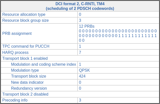
This DCI is a PDSCH scheduling for Transmission Mode 4, which corresponds to closed-loop spatial multiplexing. In this mode, two codewords can be transmitted simultaneously over 2 antenna ports by using a precoding matrix which is indicated in the DCI. In this case, only one codeword is enabled, so the same codeword is sent simultaneously over the two antenna ports. The precoding codebook index is 3, which corresponds to the precoding matrix \([1, i]/\sqrt{2}\). This simply means that the codeword is transmitted with a 90º phase advance in port 1, with respect to port 0.
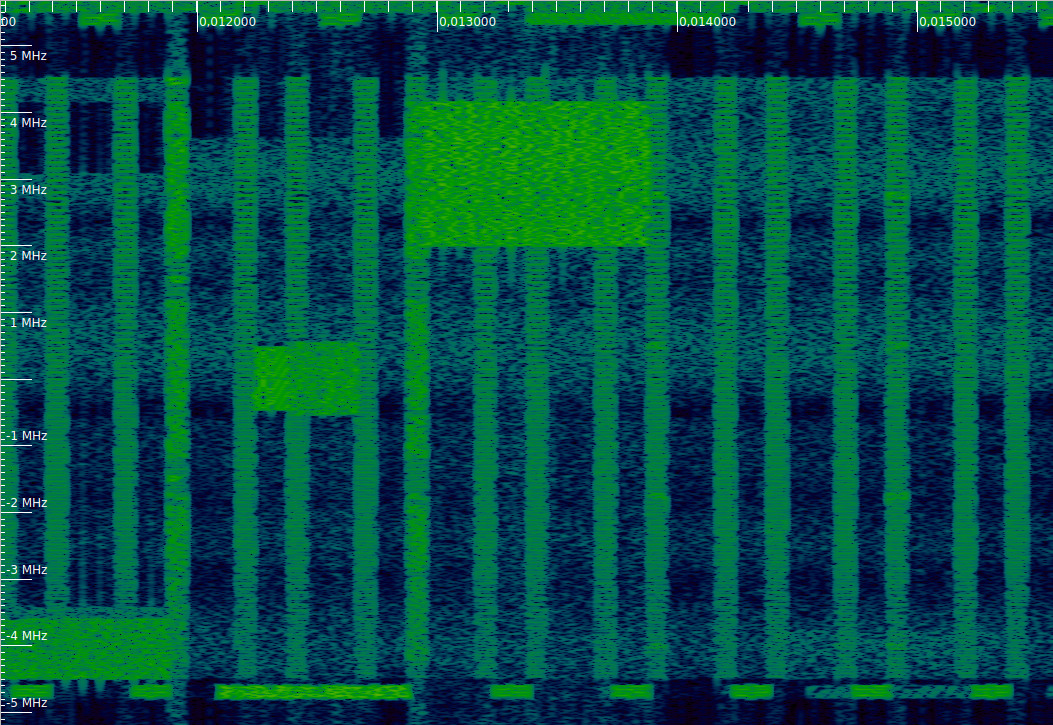
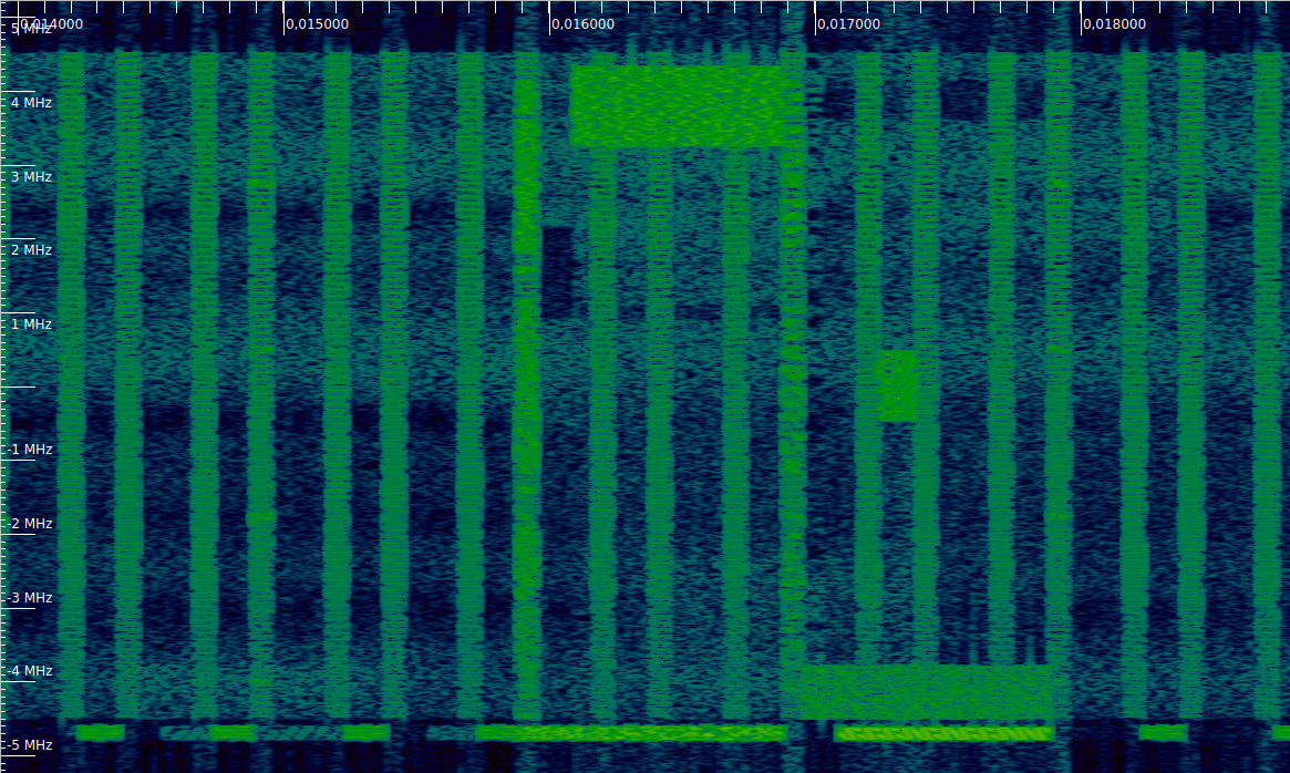
The waterfall corresponding to this DCI can be seen below. The DCI is transmitted slightly before 0.013 seconds, and then we can see the PDSCH transmission in the upper resource blocks of the cell. Note that the resource blocks used match those indicated in the DCI.
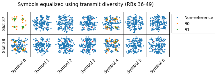
In a previous post I equalized the PDSCH transmissions with transmit diversity. For some of the transmissions I didn’t obtain a good constellation. I suspected that a different transmission mode was used for these. Below we can see the corresponding constellation plots for this PDSCH transmission. Now we know this transmission doesn’t use trasnmit diversity, but rather spatial multiplexing of one codeword over two antenna ports. In a future post I will try to use the correct equalization for these PDSCH transmissions.
There are other DCIs identical to this one in subframes 31, and 52. The constellations of the PDSCH symbols also look similar. Thus, we see that the UE with C-RNTI 0xc33c is not only uplinking data during this time interval, but also downlinking some data.
Yet another DCI is in subframe 16. It is addressed to the SI-RNTI. It is a DCI format 1A carrying PDSCH scheduling using a few of the lower resource blocks of the cell, similarly to the P-RNTI DCIs that we’ve seen. A similar SI-RNTI DCI occurs also in subframe 36, so it seems that some system information is sent every 20 ms.
Finally, the most intersting DCIs are two format 2 DCIs addressed to C-RNTI 0xced8. They occur in subframes 18 and 32. The figure below shows the DCI from subframe 18. It is a Transmission Mode 4 PDSCH scheduling which uses two codewords for simultaneous transmission over 2 antenna ports. An additional interesting feature is that the resource block assignment is spread over two segments: the lower and the upper parts of the cell.
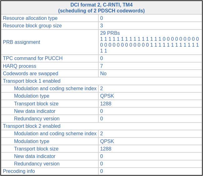
The waterfall corresponding to this DCI is shown here. We can see the two segments of resource blocks used by the PDSCH.
When I tried to equalize these PDSCH transmissions with transmit diversity, the results were horrible. The constellation plots are shown below, separately for the lower and upper sets of resource blocks. The effects of the two-codeword spatial diversity on the constellation are clear. I don’t think it’s possible to separate the two codewords with just a single receive antenna, which is what we have in this recording.

The next PDSCH scheduling for C-RNTI 0xced8 (in subframe 32) also uses a distributed resource block allocation, but only carries a single codeword.
This finishes the summary of all the DCIs found in the first 50 subframes of the recording. It is convenient to mention that there are some PDSCH transmissions that do not have a corresponding DCI. One of these is shown in the waterfall below. These PDSCH transmissions always start on the fourth symbol of the subframe, regardless of the CFI value. They are transmissions for BL/CE UEs.
The BL/CE UEs can only receive 1.4 MHz of bandwidth simultaneously. Therefore, these UEs do not use the PDCCH, as it is spread over all the cell bandwidth. Additionally, their PDSCH transmissions start later in the subframe in order to leave a guard time for frequency retuning. I observed these transmissions first in the post about transmit diversity equalitzation.
Code and data
I have extended the Jupyter notebook from the previous posts to include the calculations and plots that have been presented in this post. The recording that I am using is, as in the rest of the series of posts about the LTE dowlink, the LTE_downlink_806MHz_2022-04-09_30720ksps SigMF recording in my LTE recordings folder.
You are using a USRP, is it possible to a LimeSDR instead? I have used the LIMESDR with the Lime Tools LTEscan sw. I was able to recover the Master Information Block (MIB) but interestingly enough only at 806 MHz. Is this a coincidence. Also to get the SIB1 data how many frames should we capture?
Hi Kurtul, yes, it is possible to use a LimeSDR for this. It supports more or less the same sample rates as the USRP.
Regarding the 806 MHz carrier frequency, this will be dependent on how the band B20 is sold out to the different companies in your area. The only restriction that LTE places on the carrier frequency is that it should correspond to an EARFCN.
Regarding the SIB1, see this. A transport block for the SIB1 is sent in subframe 5 every other radio frame (i.e., every 20 ms). Each SIB1 is sent in 4 transport blocks using different redundancy versions, so the SIB1 transmission period is 80 ms. I think that the SIB1 can be decoded from a single (any one) of these 4 transport blocks, so if you’re not time-aligned to the eNB, you should record a minimum of 21 ms to make sure that you record one of these SIB1 transmissions.
Linking with the contents of the post, the SIB1 transport blocks are those using the SI-RNTI 0xffff. They appear in subframes 16 and 36 (I have numbered the subframes according to the order in which they appear in the recording; these subframes are actually the 5th subframes in their corresponding radio frames). Their DCI indicates a transport block size of 176 using 4 PRBs starting at PRB 0. The two DCIs indicate redundacy versions 2 and 3 respectively.
That was extremely helpful. I understand the SIB1 blocks are already in the recording. Do you have a suggestion on an open source tool to decode them?
I guess that srsRAN is able to decode them. I was planning to decode them manually with some Python, as done in these posts, but I’m falling quite behind on that project.
Hi Daniel,
Great stuff, as always.
If I am interested in finding the Uplink grant (UL resource allocation), I should look for DCI format 0. But I do not know in which subframe it will be found. So, what is the best method: capture large number of subframes, decode all the DCIs there are and hope that one of them is format 0. Is that correct?
Thanks for great explanation.
Hi Sohail, that’s correct. I cannot think of a cleverer or easier way to locate DCI format 0’s than to decode all the DCIs. You don’t need to record/decode that much length. If a UE is connected and trying to uplink some data, it will get uplink grants periodically.
Great. Thanks sir.