In one of my previous posts about Voyager 1, I stated that the Voyager probes used as forward error correction only the k=7, r=1/2 CCSDS convolutional code, and that Reed-Solomon wasn’t used. However, some days ago, Brett Gottula asked about this, citing several sources that stated that the Voyager probes used Reed-Solomon coding after their encounter with Saturn.
My source for stating that Reed-Solomon wasn’t used was some private communication with DSN operators. Since the XML files describing the configuration of the DSN receivers for Voyager 1 didn’t mention Reed-Solomon either, I had no reason to question this. However, the DSN only processes the spacecraft data up to some point (which usually includes all FEC decoding), and then passes the spacecraft frames to the mission project team without really looking at their contents. Therefore, it might be the case that it’s the project team the one who handles the Reed-Solomon code for the Voyagers. This would make sense specially if the code was something custom, rather than the CCSDS code (recall that Voyager predates the CCSDS standards). If this were true, the DSN wouldn’t really care if there is Reed-Solomon or not, and they might have just forgotten about it.
After looking at the frames I had decoded from Voyager 1 in more detail, I remarked that Brett might be right. Doing some more analysis, I have managed to check that in fact the Voyager 1 frames used Reed-Solomon as described in the references that Brett mentioned. In this post I give a detailed look at the Reed-Solomon code used by the Voyager probes, compare it with the CCSDS code, and show how to perform Reed-Solomon decoding in the frames I decoded in the last post. The middle section of this post is rather math heavy, so readers might want to skip it and go directly to the section where Reed-Solomon codewords in the Voyager 1 frames are decoded.
The Voyager Reed-Solomon code
One of the references that Brett gave is the paper Reed-Solomon Codes and the Exploration of the Solar System, by McEliece and Swanson. This is a rather interesting paper from 1993 that gives a historic overview of the use of Reed-Solomon codes in deep space missions. In Section 3.1 it speaks about the Voyager mission. The summary is that the convolutional code was a fine solution for the transmission of uncompressed digital images, as these could tolerate a relatively high BER. However, some advances in compression theory made it possible to implement compression on-board and transmit compressed images. These required a much lower BER, so using concatenated coding with a Reed-Solomon outer code was an attractive solution. The image compression and concatenated coding were deemed too risky for the main mission to Jupiter and Saturn, but they were used for the extended mission after the Saturn fly-bys.
The paper gives a detailed description of the Reed-Solomon code used by the Voyagers. As we will see, I may describe it as “the first Reed-Solomon code that one could think of”. This predates the CCSDS Reed-Solomon code, and it is interesting to see how the Voyager Reed-Solomon code later evolved into the CCSDS code.
The Voyager Reed-Solomon code uses the field \(GF(2^8)\), so that the codewords have \(n = 255\) bytes. The number of parity check symbols was 32, so that up to \(E=16\) byte errors could be corrected, and the code was a (255, 223) linear code, just like the current CCSDS code. These code parameters may seem too natural nowadays, but perhaps Voyager was one of the first missions to use them. For instance, the same paper mentions that Mariner used a (6, 4) code over \(GF(2^6)\). The paper doesn’t explain exactly why these parameters were chosen. Working with \(GF(2^8)\) might seem reasonable in byte-oriented computers. Usually a Reed-Solomon code over \(GF(2^8)\) will have \(n=255\). However, the choice to correct up to \(E=16\) byte errors might have been somewhat arbitrary.
The field \(GF(2^8)\) is constructed by using the primitive polynomial\[p(x) = x^8+x^4+x^3+x^2+1,\]which the paper mentions to be the first one of degree 8 in the tables of irreducible polynomials given in Appendix C in the book Error-Correcting Codes, by Peterson and Weldon. The generator polynomial of the Reed-Solomon code should have as roots 32 consecutive powers of a primitive element. The chosen generator is the obvious one,\[g(x) = (x-\alpha)(x-\alpha^2)\cdots(x-\alpha^{32}),\]where \(\alpha\) is a root of \(p(x)\). This is a valid choice because since \(p(x)\) is a primitive polynomial, then \(\alpha\) is a primitive element in \(GF(2^8)\).
It is interesting to see how this code is still in use nowadays, since it has probably ended up in many popular Reed-Solomon libraries. For instance, a quick search in gr-satellites shows that exactly the same Voyager code is used in the cubesat 3CAT-1, and variations with a different error correction capability are used in ESEO and TT-64 (\(E=8\)), Swiatowid (\(E=5\)), and ÑuSat (\(E = 2\)). All the other satellites supported in gr-satellites that use Reed-Solomon use the (255, 223) CCSDS code, either with the conventional or dual basis.
The CCSDS Reed-Solomon code
Even though it is somewhat of a diversion from the main topic of this post, it is interesting to see what changes in the Voyager Reed-Solomon code lead to the current CCSDS Reed-Solomon code, which is defined in Section 4 of the TM Synchronization and Channel Coding Blue Book. The CCSDS code was the result of a series of optimizations done by Berlekamp with the goal of obtaining a code that had the same error correction properties as the Voyager code, but for which much simpler encoders could be built in hardware. The JPL report Reed-Solomon Encoders – Conventional vs Berlekamp’s Architecture gives a detailed explanation of these changes.
The CCSDS Reed-Solomon code is also a (255, 223) code over \(GF(2^8)\). The first difference with respect to the Voyager code is really customary. In the CCSDS code, the field \(GF(2^8)\) is defined using the primitive polynomial\[q(x) = x^8 + x^7 + x^2 + x + 1\]instead of the polynomial \(p(x)\) given above. However, the root \(\beta\) of \(q(x)\) is only used indirectly to define other elements of \(GF(2^8)\), which are really the ones that determine the code. Therefore, the same code could have been defined using any other irreducible polynomial of degree 8 to define \(GF(2^8)\). Note two caveats: First, this remark is only true when using the dual basis (which is one of Berlekamp’s central ideas); when using the conventional basis, the element \(\beta\) is used to encode the field elements as 8 bit numbers, so a different choice of \(q(x)\) would give a different code. Second, here we are using \(\beta\) in order to distinguish the root of \(q(x)\) from \(\alpha\), the root of \(p(x)\) in the Voyager code. In the CCSDS documentation \(\beta\) is used to denote another field element (we will use \(\delta\) below to denote that field element).
The first main idea of Berlekamp is that instead of constructing the generator polynomial of the code using the powers \(\gamma\), …, \(\gamma^{32}\) of a field element \(\gamma\) (as done in the Voyager code), if we use\[h(x) = (x-\gamma^{112})(x-\gamma^{113})\cdots(x-\gamma^{143}),\]then \(h(x)\) is a palindromic polynomial, meaning that \(x^{32}h(1/x) = h(x)\). This happens because the roots of \(h(x)\) are pairwise inverses, i.e., \(\gamma^{112} = \gamma^{-143}\), \(\gamma^{113} = \gamma^{-142}\), etc.
Having a palindromic polynomial as the code generator is helpful because the encoder works by multiplying field elements by each of the coefficients of the code generator polynomial. Since palindromic polynomials have pairwise equal coefficients, we save half of the multiplications. Therefore, making the 32 consecutive powers of \(\gamma\) be symmetric about 127.5, rather than about 16.5 (which is what happens if we use \(\gamma\), \(\gamma^2\), …, \(\gamma^{32}\)) is advantageous to simplify the encoder.
Another remark that we have used tacitly is that it is not necessary to use a root of the polynomial that generates the field (\(\beta\) in the case of \(q(x)\)) to construct the roots of \(h(x)\) using consecutive roots. In fact, it is possible to choose any \(\gamma\) that is a primitive field element, as we have done above. Berlekamp will use this freedom to his advantage.
The second key idea of Berlekamp, and what is probably the most ingenious aspect of his Reed-Solomon code optimization, is the use of the dual basis. If \(\delta\) is a field element that doesn’t belong to \(GF(2^4)\), then the elements \(1\), \(\delta\), \(\delta^2\), …, \(\delta^7\) form a basis for \(GF(2^8)\) as a linear space over the prime field \(GF(2)\). There is a dual basis \(\ell_0\), \(\ell_1\), …, \(\ell_7\) defined by the property that \(\operatorname{Tr}(\ell_j \delta^k)\) equals 1 when \(j = k\) and 0 otherwise. Here \(\operatorname{Tr}\) denotes the field trace defined by\[\operatorname{Tr}(x) = \sum_{j=0}^7 x^{2^j} \in GF(2)\]for \(x \in GF(2^8)\).
We can use the dual basis to represent an element \(x \in GF(2^8)\) as a linear combination\[x = z_0\ell_0 + z_1 \ell_1 + \cdots + z_7\ell_7,\]with \(z_j\in GF(2)\). The coefficients \(z_j\) can be computed as \(z_j = \operatorname{Tr}(x\delta^j)\).
An interesting property of the dual basis is that the multiplication by \(\delta\), which defines a \(GF(2)\)-linear operator on \(GF(2^8)\), has a simple expression in the coordinates given by the dual basis. The element \(\delta^8\) can be written in terms of \(1\), \(\delta\), …, \(\delta^7\) as\[\delta^8 = c_0 + c_1\delta + c_2\delta^2 + \cdots + c_7\delta^7.\]This implies that\[x\delta = z_1\ell_0 + z_2\ell_1 + \cdots + z_7\ell_6 + (c_0z_0 + c_1z_1 + \cdots c_7z_7)\ell_7.\]Thus, given the dual basis coordinates of \(x\), to compute the dual basis coordinates of \(x\delta\) we just need to left shift the coordinates and use a linear map to compute the new component that is shifted in.
Compare this with what happens if we instead use coordinates with respect to the basis \(1\), \(\delta\), …, \(\delta^7\). Then, if\[x = u_0 + u_1 \delta + u_2 \delta^2 + \cdots u_7 \delta^7,\]we have\[x\delta = u_7c_0 + (u_0 + u_7c_1)\delta + (u_1 + u_7c_2)\delta^2 + \cdots + (u_6 + u_7c_7)\delta^7.\]Thus we see that to compute the coordinates of \(x\delta\) from the coordinates of \(x\) we need perform a right shift of the coordinates followed by adding \(u_7\) multiplied by a vector that depends only on \(\delta\).
There is a nice way to relate the expressions for the operator of multiplication by \(\delta\) in the dual and conventional bases: since this operator is self-adjoint, its matrix with respect to the dual basis is the transpose of its matrix with respect to the conventional basis (we say that a \(GF(2)\)-linear map \(A\) on \(GF(2^8)\) is self-adjoint if \(\operatorname{Tr}(A(x)y) = \operatorname{Tr}(xA(y))\) for all \(x\) and \(y\) in \(GF(2^8)\)).
Note that the operator of multiplication by \(\delta\) in these two bases is related to the theory of linear feed-shift registers. In fact, the multiplication by \(\delta\) in the dual basis gives the transition map for the Fibonacci form of an LFSR, while the multiplication in the conventional basis gives the transition map for the Galois form of an LFSR. Using this, we see that the output of the Fibonacci LFSR at step \(n\) is \(\operatorname{Tr}(x_0\delta^n)\), where \(x_0\) is the reset state (encoded in dual basis coordinates in the register), while the output of the Galois LFSR at step \(n\) is \(\operatorname{Tr}(y_0\delta^n\ell_7)\), where \(y_0\) is the reset state (encoded in the conventional basis in the register). This gives us that the relation required to generate the same sequence with the Fibonacci and Galois forms of the LFSR is \(x_0 = y_0 \ell_7\) (taking into account that each element should be written in the correct basis in the register).
Now let us see what happens when we consider the operator of multiplication by a fixed element \(g\in GF(2^8)\). This is the basic operation that the Reed-Solomon encoder performs, taking as \(g\) each of the coefficients of the code generator polynomial. As above, we consider the multiplication by \(g\) as a \(GF(2)\)-linear map on \(GF(2^8)\). Working in dual basis coordinates, we know that\[xg = \operatorname{Tr}(xg)\ell_0 + \operatorname{Tr}(xg\delta)\ell_1 + \operatorname{Tr}(xg\delta^2)\ell_2 + \cdots + \operatorname{Tr}(xg\delta^7)\ell_7.\]Now, the functional that sends \(x\) into \(\operatorname{Tr}(xg)\) can be written in coordinates with respect to the dual basis as\[\operatorname{Tr}(xg) = a_0z_0 + a_1z_1 + \cdots + a_7z_7,\]where\[x = z_0\ell_0 + z_1 \ell_1 + \cdots + z_7\ell_7,\]and \(a_0,\ldots,a_7\in GF(2)\) depend only on \(g\) (in fact \(a_j = \operatorname{Tr}(g\ell_j)\) are the coordinates of \(g\) with respect to the conventional basis). This expression for \(\operatorname{Tr}(xg)\) is simple to compute in digital logic, provided that the input element \(x\) is already given to us in dual basis coordinates.
To compute \(\operatorname{Tr}(xg\delta)\), we replace \(x\) by \(x\delta\), using the formula given above to compute the dual basis coordinates of \(x\delta\) from the dual basis coordinates of \(x\), and then apply the formula for \(\operatorname{Tr}(xg)\). Proceeding iteratively in the same manner, we can compute \(\operatorname{Tr}(xg\delta^2)\), …, \(\operatorname{Tr}(xg\delta^7)\). These are the coordinates for \(xg\) in the dual basis, which is what we wanted to compute.
Thus, we have seen that when we have the dual basis coordinates for \(x\), there is a simple way to compute the dual basis coordinates for \(xg\). This is Berlekamp’s key idea for reducing the digital logic usage of a Reed-Solomon encoder. Note that in a Reed-Solomon encoder we need to compute \(xg_0\), …, \(xg_{32}\), where \(g_j\) are all the coefficients of the generator polynomial. Each of these will have its own dedicated expression to compute \(\operatorname{Tr}(xg_j)\), but then the passage from \(x\) to \(x\delta\) can be shared between all the computations, since it does not depend on \(g_j\).
It is worth spending a moment to see why this kind of approach needs the dual basis, and doesn’t really work if we use coordinates with respect to the basis \(1\), \(\delta\), …, \(\delta^7\) instead. In this case we have\[xg = \operatorname{Tr}(xg\ell_0) + \operatorname{Tr}(xg\ell_1) \delta + \operatorname{Tr}(xg\ell_2) \delta^2 + \cdots + \operatorname{Tr}(xg\ell_7)\delta^7,\]and\[x = u_0 + u_1 \delta + u_2 \delta^2 + \cdots + u_7 \delta^7,\]where \(u_j = \operatorname{Tr}(x\ell_j)\). As before, we could compute \(\operatorname{Tr}(xg\ell_0)\) as a linear combination of the coefficients \(u_j\). However, to compute the next trace we need, \(\operatorname{Tr}(xg\ell_1)\), if we want to apply the same linear combination we would need to replace \(x\) by \(x\ell_1\ell_0^{-1}\). This not only doesn’t have a simple expression in coordinates, but also is not the same calculation that when we need to replace \(y = x\ell_1\ell_0^{-1}\) by \(y \ell_2\ell_1^{-1}\) in order to compute \(\operatorname{Tr}(xg\ell_2)\) (and so on for all the other traces we need to compute).
The final optimization done by Berlekamp consists in noticing that \(\gamma\) can be chosen to be any primitive element in \(GF(2^8)\) (there are \(\varphi(255) = 128\) such elements, where \(\varphi\) denotes Euler’s totient function), and \(\delta\) can be chosen to be any element in \(GF(2^8)\setminus GF(2^4)\) (there are 240 such elements). By performing a computer aided search, he selected a \(\gamma\) and \(\delta\) that minimized the digital logic gates required to perform the calculations for the multiplication operators by \(g_0\), …, \(g_{32}\) in the dual basis coordinates. He settled on \(\gamma = \beta^{11}\) and \(\delta = \beta^{117}\). These choices have been maintained in the CCSDS Reed-Solomon code.
Reed-Solomon codewords in the Voyager frames
The paper by McEliece and Swanson states that Voyager uses an interleaving depth of 4 in its Reed-Solomon frames. However, the paper doesn’t mention how much virtual fill is used to shorten the Reed-Solomon codewords. Observe that it is necessary to have some shortening, because 4 interleaved (255, 223) Reed-Solomon codewords amount to a total of 8160 bits, while the Voyager 1 frames that I decoded in last post have only 7680 bits (including the ASM). I haven’t found any source mentioning how much amount of virtual fill is used in the Voyager 1 frames. However, it is not too difficult to find the correct virtual fill with some trial and error.
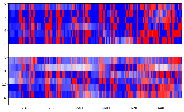
Indeed, if we look at the raster plots of the frames I decoded in the previous post, it is easy to find where the Reed-Solomon parity check bytes are. The parity check bytes look much more random than the rest of the data, and they can be spotted visually. The figure below shows the parity check bytes starting at around bit 6625. Compare the structured data before this point with the rather random data afterwards.
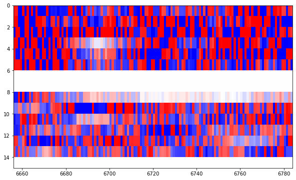
We continue through several figures containing 128 bits of random looking Reed-Solomon parity check bytes, like this.
Until we arrive to the final figure, where the Reed-Solomon parity check bytes end at around bit 7650 and we have some rather deterministic bits afterwards.
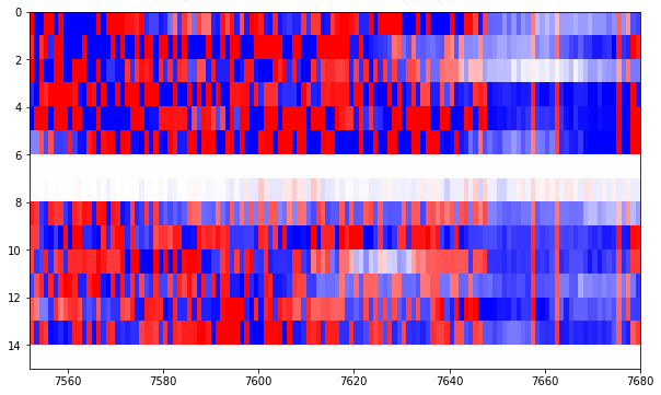
Thus, in total, we see that we have approximately 7650-6625 = 1025 bits worth of Reed-Solomon parity check bytes. This is just what we expected, since 32 bytes times 4 interleaved codewords equals 1024 bits.
The last portion of the frame is approximately 30 bits long (from 7650 to 7680). Therefore, we assume that it is really 32 bits long, and so the last 4 bytes of the frame do not form part of the Reed-Solomon codewords.
The question now is where do the Reed-Solomon codewords start. At the beginning of the frame we have two repetitions of the 32-bit ASM. Typically these do not form part of Reed-Solomon codewords, since they are a fixed pattern that doesn’t need to be error corrected (for instance, in CCSDS, the ASM is outside of the Reed-Solomon codeword). Therefore, the question is basically how many bytes we need to throw away from the beginning of the frame in order to be left with just the 4 interleaved Reed-Solomon codewords. The amount of bytes that we throw should be a multiple of 4 bytes, so that the 4 interleaved codewords have the same length.
Here is where we use trial and error. If we make a small mistake in the size of the Reed-Solomon codewords, the decoder will correct our mistake as corrected byte errors. For instance, if we include an extra byte, then we are typically supplying a non-zero data byte instead of a zero byte as virtual fill. The decoder will correct this byte to a zero. Conversely, if we miss a byte, we are supplying a zero byte as virtual fill instead of a data byte which is typically non-zero. The decoder will correct this zero to the correct data value. See my post about a Reed-Solomon bug in Queqiao for some related things we can do with Reed-Solomon codes.
Thus, by changing the codeword size to try to minimize the number of Reed-Solomon decoder byte errors (and striving to get zero errors), we can find the correct codeword size. My initial guess was that the first 128 bits of the frame (which amounts to 4 bytes for each of the 4 interleaved codewords) didn’t form part of the Reed-Solomon codewords, since these contain two repetitions of the ASM and some counters. However, it turns out that the the Reed-Solomon codewords start right at the beginning of the frame. They even include the ASMs.
Therefore, only the last 4 bytes of the frame are not part of the Reed-Solomon codewords. The remaining 7648 bits are 4 interleaved (239, 207) Reed-Solomon codewords.
I have used a Jupyter notebook and Phil Karn KA9Q’s libfec to find the correct codeword size and decode the Reed-Solomon frames. The number of corrected bytes in each of the frames of each recording is listed below (each row lists the byte errors of each of the 4 interleaved codewords corresponding to a frame).
Recording 11
[ 1,  3,  0,  0]
[ 1,  0,  0,  0]
[ 1,  1,  0,  0]
[ 0,  1,  0,  0]
[ 2,  2,  2,  1]

Recording 15
[ 3,  2,  2,  1]
[ 7,  7,  5,  4]
[ 2,  6,  6,  3]
[ 2,  2,  2,  1]
[ 0,  1,  1,  0]
We see that in all the frames that appear fully in the recording (some frames are cut short at the beginning and end of each recording) all the byte errors can be corrected and the frames can be successfully decoded. We also note again that the SNR of recording 11 is better, since there are fewer byte errors. Since we get zero byte errors in several of the codewords, we know we are using the correct codeword size.
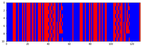
After successful Reed-Solomon decoding, we are sure of the correct values of each of the bits in the Reed-Solomon codewords, so we can now pass from the soft bits we used in the last post to hard bits that only have the values 0 and 1. The raster plots now look like this one, which shows the first 128 bits of the frames. I have thrown away those frames which couldn’t be decoded by the Reed-Solomon decoder.
Since the last 32 bits of the frame do not form part of the Reed-Solomon codeword, we cannot error correct those, so I have left the soft bits there. The result looks like this.

The Jupyter notebook contains all the plots of the Reed-Solomon corrected frames. Now it should be slightly easier to look carefully through the data to try to find patterns.
Fantastic work! I appreciate the insights into the evolution from the Voyager code to the CCSDS code. For a long time I had thought that they were the same. The CCSDS rate 1/2 convolutional code is often referred to as the “Voyager code,” and since I knew Voyager pioneered the use of RS + CC I had just assumed that both codes were unchanged in CCSDS.
Now that you’ve figured out the outer code structure it would be neat to try Travis Fisher’s idea to attempt to correlate against some of the published science data. If I find time one of these days I might try to dig up data from the relevant timeframes. That in itself might be a tedious project…
I’ve also tried to find further references on Voyager frame structure online but haven’t come across much. This document has some interesting detail on the hardware design of the Flight Data System, which is interesting but no direct insight on frame structure: https://history.nasa.gov/computers/Ch6-2.html. One important reference it cites is “Design of a CMOS Process for Use in the Flight Data Subsystem of a Deep Space Probe” by John “Jack” L. Wooddell circa 1974. It describes this as “a paper for a graduate computer science course taught by Dr. Melvin Breuer at the University of Southern California” and is apparently a pretty detailed description of the flight design of the FDS (!!). I wasn’t able to find it online. Frame structure details are probably mostly if not all in software, but since this was such a special purpose computer there may be some interesting clues in such a paper about its capabilities and limitations.
Brett
Some diagrams of Voyager frame structure are shown in
“Voyager image data compression and block encoding”
M G Urban 1987
https://repository.arizona.edu/bitstream/handle/10150/615317/ITC_1987_87-0821.pdf?sequence=1
Hi Vince, thanks for the reference! I hadn’t seen it. At a glance it mostly speaks about image transmission, which is probably not the kind of data being transmitted here, but certainly very interesting. I’ll try to read this in full later.
Hi Daniel – you suggest that the decision to correct up to 16 errors in the Voyager Reed-Solomon code might have been somewhat arbitrary. This wasn’t the case. Odenwalder, who designed the concatenated code combining the (7,1/2) rate convolutional code and the R-S code experimented with many different parameters. In his 1976 book/paper “Error Control Coding” ( https://apps.dtic.mil/sti/pdfs/ADA156195.pdf ) you can see (between pages 196-198) in Figures 7.3 and 7.4 that the bit error rate curves for E=16 are superior to E=8 and E=24, (with a AWGN noise channel with BPSK or QPSK modulation). Interestingly, 9 bit codewords give better performance than 8, but presumably were more expensive in coding hardware complexity.
Hi Vince, I don’t know why I didn’t reply to your comment before. You’re absolutely right. I should have imagined that someone would have done a study and optimized E to give the best Eb/N0 performance. What I found interesting in those plots is that there is a large gap between E=8 and E=16, but E=16 and E=24 are close by. That makes me wonder whether there is some other choice which is slightly better than E=16, such as E=14 or E=18.
“9 bit codewords” should read “9 bit symbols”, sorry.
I think this explains why the ASM appears twice, it’s transmitting the data off the tape which is stored as frames, but since a frame includes the header bytes/ASM with the RS, it needs to send the whole thing.. (although arguably they could chop the ASM as it’s fixed but perhaps that was just adding more code into very limited memory and they opted to leave it raw)
Hi Stephen, that makes a lot of sense. In old spacecraft, sending recording telemetry would usually be the simplest kind of tape playback.
Hi – Minor correction Jack Wooddell is not named John. He is my uncle, son of Larry Wooddell of Kent Ohio (black squirrels and arborist at KSU). A long term JPL employee, he still lives in La Canada. I know a little about his accomplishments from the internet as my uncle is very modest and would never brag. He understates the accomplishments.
Thanks for the correction! I was wondering how could Brett Gottula have possibly made that mistake, since when he mentioned ‘John “Jack” L. Wooddell’, it seemed that he was quoting literally some reference.
I looked closely at the report he mentioned: https://ntrs.nasa.gov/api/citations/19880069935/downloads/19880069935_Optimized.pdf Certainly, Wooddell is first mentioned as Jack L. Wooddell in page 180, and then as J. Wooddell or Wooddell alone. However there is an “Interview with John Wooddell, Jet Propulsion Laboratory, May 21 1984” that appears in pages 338 and 375, and John Wooddell also appears in the acknowledgements. A different person? A mistake that got replicated in 3 places? I haven’t found ‘John “Jack” L. Wooddle’ written like so anywhere.
I used to talk to Jack Wooddell at JPL when I worked there approximately 33 years ago. I was using a computer in the same 2-man office that Jack was in. He was proud of the fact that the computer he designed was still working after traveling that long. But he did seem quite humble, sitting in an obscure, shared office in an old JPL building. I still remember his smile. I always felt honored to have met this great engineer, and always enjoy telling this little story.