In my last post I spoke about the James Webb Space Telescope telemetry, and I decoded a recording I made with the Allen Telescope Array. I used an IQ sample rate of 3.84 Msps when doing this recording because I wanted to see if there were any ranging signals. Usually, ranging signals have a bandwidth of 1.5 MHz or less in baseband, so after phase modulation, approximately 3 MHz are used. Thus, 3.84 Msps gives enough bandwidth to record the typical ranging signals.
After looking at the waterfall of the recording carefully, I saw that there are sequential ranging signals present almost all the time. This is expected. Since the recording was done 7 hours after the first correction manoeuvre, the DSN would be doing ranging to compute accurate ephemerides. Often, ranging signals are not used every time that a spacecraft is tracked, but only when the ephemerides need to be refined, such as when planning a manoeuvre or shortly after executing one.
In this post I analyse these sequential ranging signals. I still haven’t had time to publish the recordings in Zenodo. After seeing that the wideband recording is of interest, due to the presence of these signals, I’m planning to publish a shorter segment of the wideband recording (the full recording is 241 GB per polarization) and publish a decimated version of the full recording where only around 100 kHz of spectrum are present (which is enough for the telemetry signal).
Sequential ranging, as performed by the DSN, is described in this module of the Telecommunications Link Design Handbook. Briefly speaking, it involves including a tone (either a sinusoid or square wave) in the phase-modulated uplink signal, which then gets remodulated into the downlink by the spacecraft transponder, and finally its phase is measured when the downlink arrives back at a groundstation. This serves to measure two-way (or three-way) light-time delay through the spacecraft transponder.
However, since phase measurements are ambiguous, there is an ambiguity of an integer number of wavelengths in the measurement. To solve this ambiguity, rather than using a tone of a single frequency, a sequence of tones of different frequencies are transmitted successively. The frequency of each tone in the sequence is half of that of the previous tone, so the ambiguity (in distance units) is twice as large. The sequence contains as many tones as needed so that the frequency of the last tone is low enough that the ambiguity it gives is larger than the a-priori estimate on the light-time delay. This allows solving the ambiguities of all the tones and producing an unambiguous measurement. Only the first tone, which has the highest frequency, and hence the highest “resolution”, is used to produce the final measurement. The remaining tones are only used to solve the ambiguities.
Another important detail is that if we were to produce the sequential ranging signal exactly as I have described, at some point the frequency of the tones would get too low and they would interfere with the telecommand and telemetry signals. To avoid this, chopping is used after some point in the sequence. This consists in sending the product of a fixed tone in the sequence, called the chop component, and the tone that should be sent. This produces tones at the sum and difference frequencies. If the frequency of the chop component is high enough, then the resulting frequencies are also high and do not interfere with the telecommand and telemetry. Often, the first tone in the sequence, which is called the range clock, is used as chop component.
The frequency of the range clock, and hence of all the other tones, is locked coherently to the uplink carrier frequency. This is done so that the tones on the downlink are coherent with the downlink carrier (since the spacecraft uses a coherent transponder). On the groundstation receiver, the phase information from the PLL that locks to the downlink carrier can be used to derive an accurate frequency reference for the ranging tones and integrate them coherently for several seconds.
This implies that the frequencies of the tones are not nice round values. In fact, for an S-band uplink, as is the case of JWST, their frequencies are of the form \(f_n = 2^{-7-n} f_U\), where \(n \geq 0\) and \(f_U\) is the uplink frequency. Often, \(n = 4\) is chosen for the range clock to give a range clock frequency of approximately 1 MHz. The next tones in the sequence are then approximately 500 kHz, 250 kHz, etc.
The sequential ranging tones in the recording of JWST are rather weak. The waterfall below, done with inspectrum shows the spectrum around the ranging clock frequency in the phase demodulated downlink. We can see the ranging clock towards the right side of the plot. It lasts for ~8 seconds. Before it, we see the the last components of the previous sequence. These are chopped with the ranging clock, so they appear as two tones symmetric above and below the ranging clock frequency. They are harder to see because the power is split among the two tones. These components lasts for ~4 seconds.
The duration of the ranging clock is chosen to give the desired ranging precision, according to the ranging clock frequency and the SNR of the ranging tone. The duration of the remaining components is chosen long enough to give a high probability of solving the ambiguities correctly. Usually, the ranging clock is longer than the other components.
Since it is hard to see the ranging tones in the waterfall, I have made a GNU Radio flowgraph to make them easier to process and see. This flowgraph extracts a 100 Hz spectrum slice around each of the tone frequencies. The output of the flowgraph can then be processed with the appropriate FFT parameters to make the tones more visible.
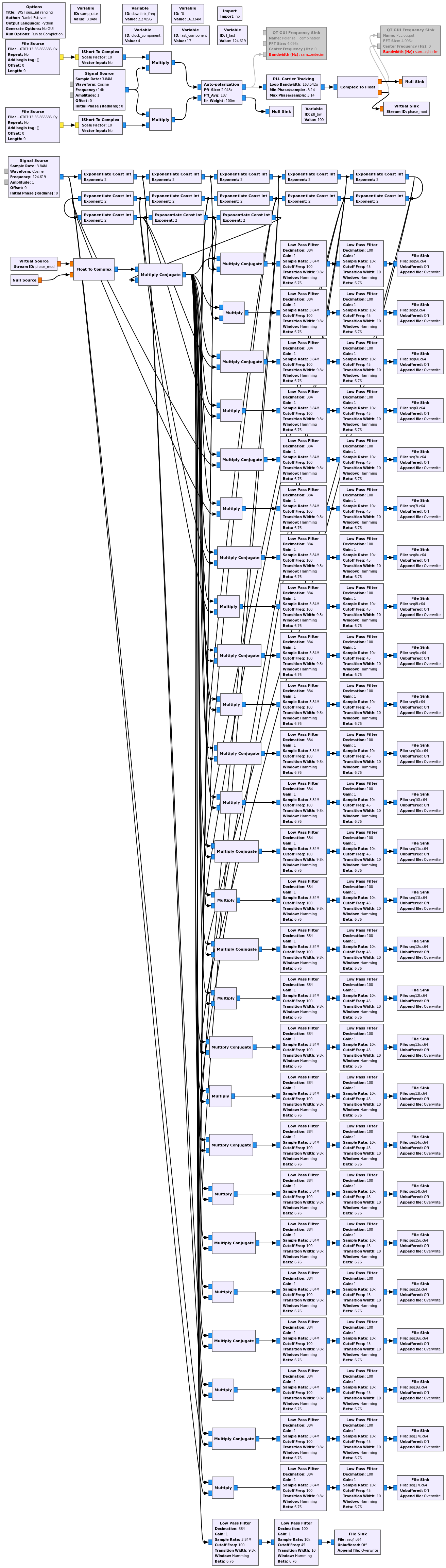
The flowgraph is a bit cumbersome, because there are many tone frequencies. JWST uses \(n = 4\) as ranging clock (~1 MHz) and the ranging sequence goes up to \(n = 17\) (~125 Hz). All the components starting with the second (\(n=5\)) are chopped with the ranging clock, so they produce two tones. Thus, there is a total of 27 tone frequencies.
To generate the local oscillators for the tone frequencies, I start with the lowest frequency one (~125 Hz) and successively square it to double its frequency until I arrive at the ranging clock. This ensures that all the local oscillators are coherent. If for instance, different Signal Source blocks were used for each of the frequencies, then rounding errors could make them non-coherent. Although in this post we will not use this coherence, because we will not measure the phase of the tones, this property could be interesting for a future study.
After mixing with the appropriate local oscillator, each of the tones is decimated from 3.84 Msps to 100 sps by using two FIR filters, performing decimation by 384 and 100.
The output of the flowgraph is processed in this Jupyter notebook. To show the ranging tones we use a 32 point FFT, giving a frequency resolution of ~3 Hz. A waterfall of each of the tones near the start of the recording is shown here.
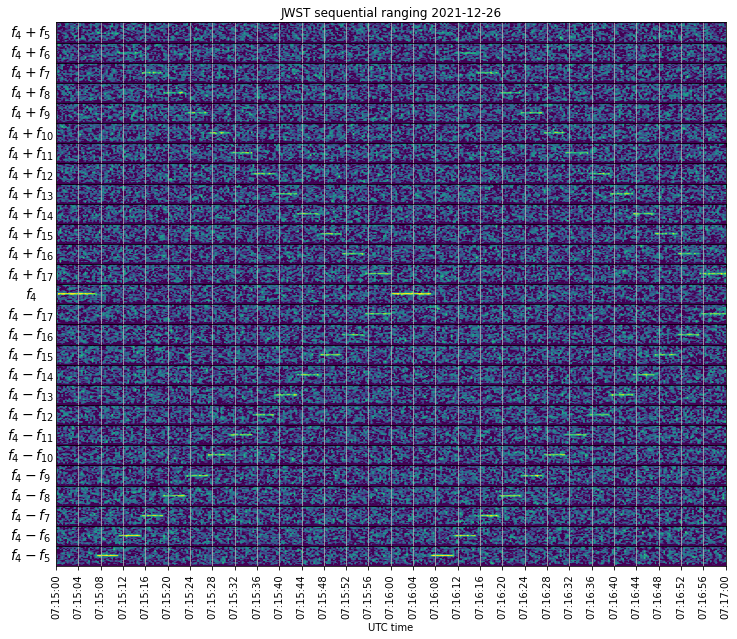
Note that all the tones are shown with the same vertical spacing in this plot, but this is just for practicality. In reality the frequency separation between each successive tone is halved, so they follow exponential curves in the waterfall, as shown above in the inspectrum plot.
We see that the full ranging sequence lasts 60 seconds. The ranging clock lasts ~8 seconds, and the remaining 13 components last ~4 seconds each. We will look at the timing more precisely below. Another thing to notice is that the upper chop tone of the second component, \(f_4 + f_5\), which is approximately 1.5 MHz, is quite weak. We will look at the power of each of the tones later, and see that this is probably due to a low-pass filter in the transmitter and/or spacecraft transponder.
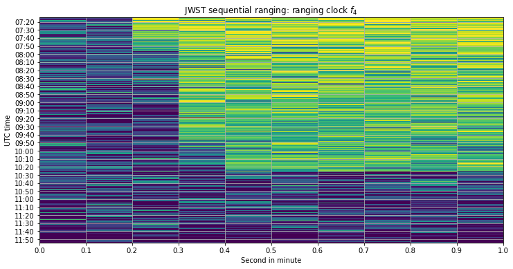
The plot shown above is not appropriate to show the data for the full recording, since the tones would be so short that they won’t be visible. To be able to show the full recording in one plot, we take advantage of the 60 second measurement cycle. First we use a 10 point FFT and use the 3 central bins to measure the power of each of the tones. Then we can plot this power in a 2D plot where each of the lines represents one minute of data and the x axis corresponds to the second within the minute. The plot for the ranging clock is shown here.
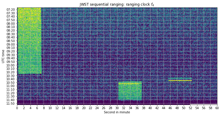
We see that the ranging clock happens at the start of the minute until approximately 10:25 UTC. Then there are no ranging clocks for some minutes, until at around 10:35 the ranging clock appears again, but now starting at ~:45 seconds in the minute. The measurement sequence is still 60 seconds long. These tones are rather weak, but then there are some very strong tones. Next, at 10:45 the position of the ranging clock shifts to :30 seconds in the minute. There are also a few very strong tones around 10:55, and the ranging continues in this manner until the spacecraft sets for ATA. The plots for the remaining tones in the sequence can be seen in the Jupyter notebook. They are similar to this one, except that each tone starts in its corresponding position in the sequence.
I think that the stop at 10:30 is due to the hand off between Goldstone and Canberra. However, it is quite interesting that the ranging timing has moved from the start of the minute.
The interesting part between approximately 10:35 UTC and 11:00 is shown below. It is apparent that there are large changes in the power of the ranging tones and that at 10:47 the sequence changes timing.

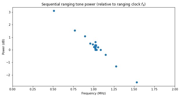
Using the data from these plots, we can measure the power of each of the tones quite accurately, using the first hour of data to average. The results are shown below. The power of all the tones except for the ranging clock has been multiplied by two to account for the fact that the total power is split in two due to chopping. We see that the power of the tones decreases with frequency, so apparently there is a low-pass filter, which is quite common.
Now let us look to the timing of the ranging tones more in detail. Keen readers might have observed in the plot of the ranging clock that its start time is moving slightly to the right. In fact, if we zoom in to the first second in the minute of this plot, this is clear, even though we only have a resolution of 100 ms in this plot.
According to the ephemerides from NASA HORIZONS, at 07:30 UTC, JWST was at 182831 km from Goldstone and 183168 km from the ATA, giving a two-way light-time of 1.221 seconds (here we are ignoring the relative motion of the spacecraft and groundstations during the signal travel time for simplicity).
In Section 2.2.4.1 in the sequential ranging documentation, the timing of the ranging signal is described. The ranging clock always starts at an integer second. Actually it starts one second before the intended transmit time \(\mathrm{XMIT}\), so that the ranging clock is already present when its reception starts (which is also done at an integer second). This matches what we see, because we are seeing the ranging clock arriving at ~0.2 seconds in the minute, so it must have been set to an intended transmission time of 0 seconds in the minute, and actually start at 59 seconds in the minute.
Four hours later, at 10:30 UTC, the distance between JWST and Goldstone was 204223 km, and the distance between JWST and ATA was 204150 km. This gives a light-time delay of 1.362 seconds, which represents an increase of 141 ms in the light-time delay. Even though we only have 100 ms resolution in the plot above, we can see that the plot is in-line with what the ephemerides describe.
Sequential ranging measures the light-time delay not by detecting when the tones start (as we are seeing here, it is not possible to do this with good resolution when the signal is weak), but rather by measuring their phase. Still, I think that the plot above is a nice demonstration of how the light-time delay increases as the spacecraft travels away from Earth.
Regarding the timing of the remaining tones, the documentation states that the ranging clock is present from \(\mathrm{XMIT} – 1\) to \(\mathrm{XMIT} + T_1 + 1\) and that then at some point within that second the next component starts. As we have seen, \(\mathrm{XMIT}\) must be 0 seconds in the minute (in the first part of the recording, when Goldstone is transmitting). Since the ranging clock duration is somewhat short of 8 seconds, we see that \(T_1 = 5\) seconds. The second component lasts until at least \(\mathrm{XMIT} + T_1 + T_2 + 2\), and then changes to the next component at some point within the following second. Since this component lasts approximately 4 seconds, we see that \(T_2 = 3\) seconds. The formula for the cycle time\[T_1 + 3 + (n_L-n_{RC})\cdot(T_2+1)\]checks out, because with these values and \(n_L = 17\), \(n_{RC} = 4\) we get 60 seconds.
To summarize, the parameters used by the JWST sequential ranging in this recording are the following.
| Ranging clock component \(n_{RC}\) | 4 |
| Last component \(n_L\) | 17 |
| Ranging clock transmit time \(\mathrm{XMIT}\) | :00, :45 and :30 |
| Ranging clock duration \(T_1\) | 5 seconds |
| Other components duration \(T_2\) | 3 seconds |
| Cycle time | 60 seconds |
| Chop component | 4 |
| First chopped component | 5 |
Thank you for the educational & interesting write-up!
There may be one or more incorrect assumptions in my question, so please advise…
I am not clear how one or more line-of-sight distance measurements is used to calculate a spacecraft’s 3-dimensional position in space. (Telling me that there are 6300 km between us doesn’t tell me whether you are in Spain or Brazil)
Can you perhaps say anything to someone not familiar with this subject about how the jump is made from a distance measurement to a position plot?
Many thanks!
@scott The antennas have a narrow beam width (on the order of 0.1 desgrees I think). The position of the spacecraft can therefore be determined by the az and el of the antenna, and the distance measured by ranging.
The DSN does not use the angular pointing of the telescope for orbit determination. For angular positioning, the Hamilton-Melbourne technique is routinely used with round-trip (2 way) Doppler, to extract the angular position from the diurnal modulation of the Doppler data.
https://descanso.jpl.nasa.gov/history/pdf/sps37-39v3_p18-23.pdf
For even higher accuracy, the DSN uses VLBI (Delta DOR in DSN speak), which gives nanoradian accuracy.
https://ipnpr.jpl.nasa.gov/progress_report/42-109/109C.PDF
Thanks for all these references! The historical documents I’m particularly interesting, since I’m more used to reading current CCSDS and 810-005 stuff.
Hi Scott,
Actually the position of the spacecraft in 3D space is not found, or at least it is not found directly. First, it is crucial that the spacecraft trajectory can’t be some random thing. If the spacecraft is not using propulsion, then it must “follow” the gravitational forces of the Sun and planets and other forces (solar radiation pressure, etc). If we were to know the position and velocity of the spacecraft (the state vector) at some instant, we could propagate (predict) the trajectory at any moment in the future or past, because it must follow these forces.
The state vector is 6 numbers (3 for position, 3 for velocity). A series of measurements that have been done at different times has potentially many numbers, even if they are the same type of measurement (for instance, here Goldstone is measuring the distance to JWST every minute for perhaps 6 hours or more). In theory, often there will only be one state vector that matches exactly this series of measurements.
In practice, there is no such thing as matching exactly, because every measurement has some error. What is done is the following. We have an a-priori estimate for the trajectory/state vector of the spacecraft (just because we don’t launch spacecraft in random directions in space). We take a series of measurements at different times. We calculate how well these measurements match the a-priori trajectory. The errors we get are called residuals. We “nudge” the trajectory a little with the hope to make the residuals smaller (math tells us how to nudge the trajectory). We keep nudging the trajectory until we make the residuals as small as we can (this is called least squares fitting). The improved trajectory we get is our new navigation solution for the spacecraft.
Also, as one can imagine, having measurements of the same type (say two range measurements) spaced by not much time (say one minute) is not very helpful, since the second measurement doesn’t tell us much new information. It is better to have measurements spaced over a wide time interval, and also measurements of different types. For this reason, two-way ranging (which measures the time that it takes for a signal to go to the spacecraft and back, which is roughly equivalent to the distance to the spacecraft) is not the only kind of measurement that is done.
Other measurements that are often used are Doppler and DDOR. With Doppler we measure something that is roughly equivalent to the relative speed between the spacecraft and groundstation. By using a very stable frequency reference on ground and locking the spacecraft’s transponder coherently to this frequency, measurements as accurate as a few milli-Hz can be done. This is equivalent to less than 1 mm/s. So we can measure spacecraft velocities very precisely.
Doppler and two-way ranging are done simultaneously any time that it is necessary to range a spacecraft, since two-way ranging just requires sending some ranging signals through the spacecraft transponder (which can be done in combination with telecommand and telemetry), and measuring Doppler is essentially for free.
DDOR involves using two groundstations that are tracking the spacecraft simultaneously, so for this reason often it is only done when necessary (because more precision is needed to plan some manoeuvres or whatever). DDOR is a form of VLBI. The difference between the times of arrivals of the signals of the spacecraft to the two groundstations is measured. A similar measurement is done for a quasar, which is used as a calibration reference. This measurement tells us something which is roughly equivalent to the relative angular position on the sky (think right-ascension and declination) of the spacecraft with respect to the quasar. The quasar absolute position is know very accurately, so in turn this tells us about the angular position of the spacecraft in the sky. DDOR is very accurate. It can give precisions better than a milli-arcsecond.
Combining all these kinds of measurements and taking measurements spaced in time, the trajectory of the spacecraft can be found quite accurately.
It is true that the DSN groundstations can also measure where they are pointing the antenna, and that their beams are relatively narrow. However, this data is often not precise enough for navigation. The antenna pointing measurement can be perhaps as accurate as 0.01 deg, but such an angle represents a very large position error at the distances that deep space probes are from Earth.
This is basically the “Mu-2” system, which replaced the earlier pseudo-random noise “Tau” spread spectrum system. I believe this sequential ranging system was not used with Mariner 9; it was definitely used with Viking Mars in 1976.
https://descanso.jpl.nasa.gov/history/pdf/tm33-768.pdf
I remember Art Zygielbaum leading the actual deployment of this system at the DSN stations in time for Viking.
The PRN system, although it is now routinely used with, e.g., GPS, was a little beyond the ability of the spacecraft transponders in the 1960s/70s, so they went “back” to sequential ranging. If the spacecraft predicts are quite good (as is common for, e.g., cruise phase) then sequential ranging is quick to perform. This presentation goes into the relative merits.
https://cwe.ccsds.org/css/docs/CSS-SM/Meeting%20Materials/2008/March-2008/DS%20Ranging%20type%20comparison%202001-11-03.pdf