BepiColombo is a joint mission between ESA and JAXA to send two scientific spacecraft to Mercury. The two spacecraft, the Mercury Planetary Orbiter, built by ESA, and the Mercury Magnetospheric Orbiter, built by JAXA, travel together, joined by the Mercury Transfer Module, which provides propulsion and support during cruise, and will separate upon arrival to Mercury. The mission was launched on October 2018 and will arrive to an orbit around Mercury on December 2025. The long cruise consists of one Earth flyby, two Venus flybys, and six Mercury flybys.
The Earth flyby will happen in a few days, on 2020-04-10, so currently BepiColombo is quickly approaching Earth at a speed of 4km/s. Yesterday, on 2020-04-04, the spacecraft was 2 million km away from Earth, which is close enough so that Amateur DSN stations can receive the data modulation sidebands. Paul Marsh M0EYT, Jean-Luc Milette and others have been posting their reception reports on Twitter.
Paul sent me a short recording he made on 2020-04-04 at 15:16 UTC at a frequency of 8420.535MHz, so that I could see if it was possible to decode the signal. I’ve successfully decoded the frames, with very few errors. This post is a summary of my decoding.
The X-band signal from BepiColombo is very similar to that of Solar Orbiter that I decoded a couple months ago, so I’ve been able to reuse most of the software. The signal is PCM/PM/Bi-φ modulated at approximately 700kbaud and uses an r=1/2 Turbo code with a block length of 8920 bits. Thus, the only difference between BepiColombo and Solar Orbiter is the baudrate (Solar Orbiter used approximately 555.5kbaud).
The SNR in this recording of BepiColombo is lower than in the Paul’s recording of Solar Orbiter, so my decoder didn’t work: the constellation locked, but it was too noisy for the Turbo decoder to correct all the bit errors. Therefore, I have tried an alternative decoding approach that seems to work better.
The decoder can be seen in the figure below. A PLL is used to track the residual carrier, phase demodulation is done, and the signal is resampled to 10 samples per symbol. After that, there is a FIR filter whose taps are a sequence of five -1’s and five +1’s. This should be thought as a matched filter to the Manchester pulse. At the appropriate sampling points, the taps of the filter are aligned with the Manchester clock and the filter wipes-off the Manchester modulation. After this we run clock recovery with the Gardner algorithm and then detect the 64bit ASM that marks the beginning of Turbo codewords.
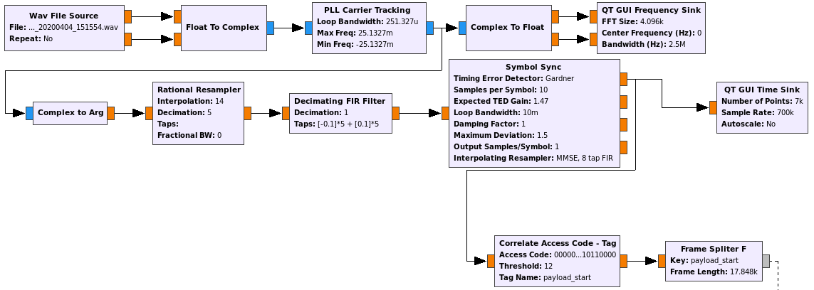
I’m not completely sure that it’s impossible for this decoder approach to false-lock at 1/2-symbol offset from the correct symbol clock, but so far it seems to work well.
The GNU Radio decoder flowgraph can be found here. As in the case of the Solar Orbiter decoder, it uses gr-dslwp for Turbo decoding, so the flowgraph is for GNU Radio 3.7, as gr-dswlp hasn’t been ported to 3.8 so far. Note that Turbo decoding is very CPU intensive, so it would be really difficult to run the decoder in real time. When I run it on my i7-2620M laptop, the demodulator goes through the recording pretty fast, but the Turbo decoder stays running for many minutes until it finishes processing all the frames.
The decoder can be seen running in the figure below. The spectrum of the in-phase and quadrature branches of the PLL-locked signal is plotted, showing clearly the phase-modulated data sidebands in the quadrature component. There are many bit errors, but even so the Turbo decoder is capable of correcting all of them.

The analysis of the decoded frames can be seen in this Jupyter notebook and the file with the decoded frames is here in case anyone wants to have a more detailed look.
A total of 1808 frames were decoded from Paul’s 46.5 second recording. Only one of these has incorrect CRC. The frames are TM Space Data Link frames. According to the master channel frame count field, only 8 frames were lost in my decoding process.
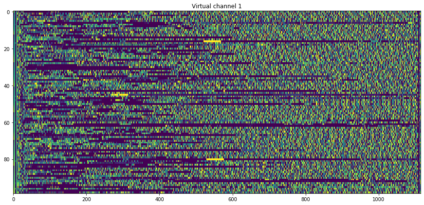
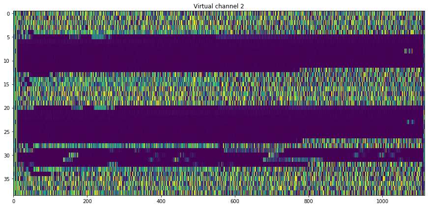
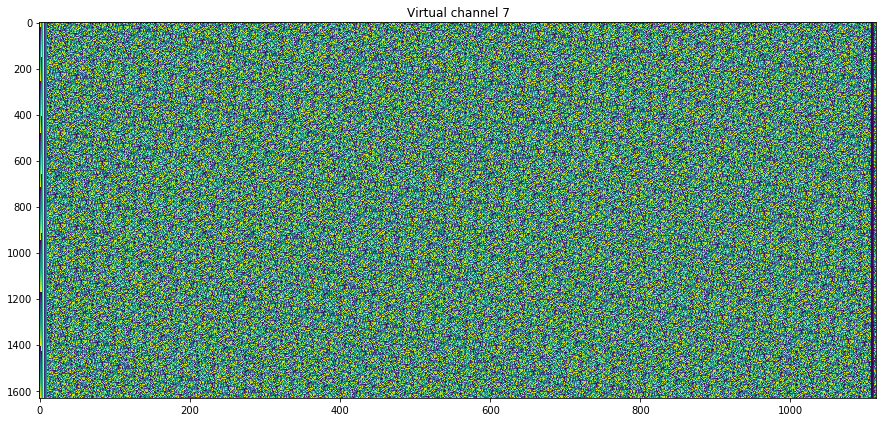
Four different virtual channels are used to transmit the data. The relative usage of these can be seen below.
Virtual channel ID 0: 38 frames
Virtual channel ID 1: 99 frames
Virtual channel ID 2: 39 frames
Virtual channel ID 7: 1631 frames
The contents of the virtual channels can be seen below. Each frame is plotted as one row of the graph, with colour-coded bytes. It can be seen that the data on each virtual channel is rather different. Virtual channel 2 is perhaps the most interesting, since it seems to have very long sequences of zeros. Virtual channel 7, where the bulk of the data is sent, shows some repetitive structure that doesn’t match the frame size.

I haven’t looked at the data in any more detail yet. What I’ve been curious about are the peaks that can be seen in the quadrature branch near the carrier. In fact, there are several peaks, as it can be seen in the figure below, which shows a close-in spectrum of the PLL-locked signal.
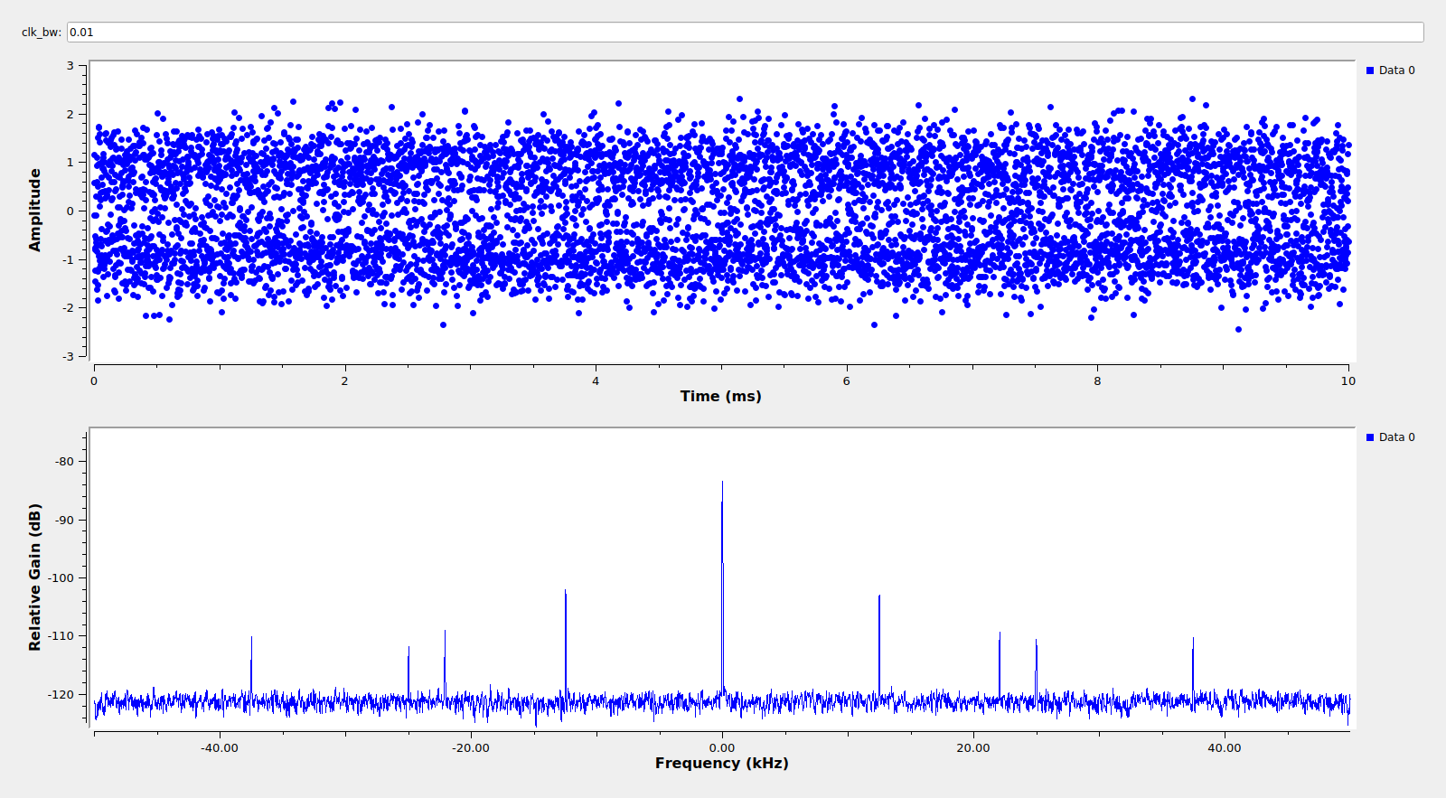
I’ve measured the frequency of these peaks to be 12490Hz, 22088Hz, 24981Hz, and 37417Hz, accurate to 1Hz or so. The last two are then 2nd and 3rd harmonics of 12490Hz. The 12490Hz and 22088Hz tones seem to be related by the fraction 4016/2271. This numerology is perhaps too much of a guess, but since 4016 and 2271 are coprime, it supports the idea that these are ranging tones. Indeed, 12490Hz/2271 is quite close to 5.5Hz (the error is 40ppm, which could be explained by Doppler and clock drift).
So my guess is that the 2271th and 4016th harmonics of a 5.5Hz clock are used for ranging. The ranging ambiguity is given by the 5.5Hz clock, and is approximately 5.5 millions of km. Regarding ranging performance, with a loop SNR of 20dB on the 22088Hz tone (which perhaps is not possible to achieve with this recording, but certainly it is not too far off), the tracking jitter of this tone would be 0.1rad RMS, which is equivalent to 216m, so this is actually not bad at all. However note that resolving the integer ambiguities would require averaging the phase jitter on the 22088Hz tone down to significantly less than 1mrad, so the SNR needed for unambiguous ranging is certainly much more than what is present in this recording.
When researching these tones I also measured the baudrate accurately by using cyclostationary analysis. It turns out that it is 699070.5 baud (accurate to around 1 baud), so I don’t think that the baudrate is related to the frequencies of these ranging tones.
More great work! Can you estimate the phase modulation index? What’s your carrier loop bandwidth and SNR? What about for symbol timing? The squaring loss can be a real challenge with turbo coding at rate r 1/6, and even at r 1/2 isn’t negligible.
Hi Phil,
The modulation index is, very approximately, 1 rad.
The PLL loop bandwidth for carrier tracking is 100 Hz. I didn’t measure the loop SNR, but it should be high: judging from the spectrum, the carrier is more than 25dB SNR in 2.5MHz with 4096 FFT bins.
For symbol timing I’m using a loop bandwidth of approx. 1kHz (If I understood the parameters of the Symbol Sync block correctly. I am convinced that it takes radians/symbol). On second thought this seems rather high, but I didn’t worry about measuring or optimizing these performance aspects. My main goal was putting together a demodulator that worked. A quick test shows that with 100Hz the loop doesn’t lock, so maybe something else is wrong.
I get your point about squaring losses. This is another case where FEC performs better than channel estimation, so the real challenge is getting the channel estimation working at the low Eb/N0 allowed by the FEC.
Your questions about performance are nevertheless quite interesting, so these go to the TODO list.
One method I’ve used for symbol timing recovery when the blocksize is fairly small, fixed and known is to drag a sync correlator across the data, find two (or more) successive frame syncs, and then divide up the interval between them into symbols with known phase and frequency. The advantage is deterministic behavior (unlike PLLs at low SNR), no squaring loss in the sync correlator and a fairly high detector output SNR, while the disadvantage is that I’m not making any use at all of the energy in the rest of the signal for symbol timing. But it has worked.
That’s quite similar to what Wei Mingchuan did for DSLWP-B in gr-dslwp. This used 250baud or 500baud, r=1/2 or 1/4 Turbo CCSDS frames with 1784 information bit frames. The receiver did symbol recovery by correlating against the ASM at the start of the frame (obtaining symbol clock phase) and then advancing the symbol clock at its nominal rate throughout the frame.
Your suggestion of using two successive ASMs (which also estimates the symbol clock rate) wasn’t used, since usually the spacecraft sent a single frame.
This approach worked very well. If you think about it, you’ll get on the order of 4000 or 8000 symbols in one of these frames. If you assume that your rate (including Doppler) is off by 1e-5, then at the end of the frame you’re still only less than 0.1 symbols off.
The only problem we found with this open loop approach was decoding through the WebSDR. The software does some weird audio resampling to keep things running smoothly, and completely breaks the hypothesis that your rate is only off by 1e-5.