This is a follow-up to my study about the Galileo broadcast clock parameters oscillations at a frequency of 1/revolution. Be advised that this short post raises more questions than answers.
In order to try to shed more light onto the possible cause of the oscillations observed in the previous post, I have now processed the broadcast ephemerides of November for all the active Galileo satellites (including the eccentric E14 and E18) except for E11 and E25, which were out of service at least for some days in November.
This post studies the amplitude and phase of the oscillations of the broadcast clocks at a frequency of 1/revolution. More formally, if we denote by \(x(t)\) the time series corresponding to either the broadcast clock bias or the broadcast clock drift, we compute the complex quantity\[\alpha = \frac{2}{T}\int_{t_0}^{t_0 + T} x(t) e^{-i[n_0(t-t_0) + M_0]}\,dt,\]where \(n_0\) denotes the mean motion in radians/second and \(M_0\) denotes the mean anomaly at \(t_0\) in radians. Note that if\[x(t) = a \cos(n_0 (t-t_0) + M_0 + \varphi),\]then \(\alpha \approx ae^{i\varphi}\), which motivates the definition of \(\alpha\).
When computing \(\alpha\) from the broadcast ephemerides, the mean motion \(n_0\) is taken as the average mean motion among all the ephemerides, while the mean anomaly \(M_0\) is taken as the mean anomaly at the first ephemeris. Note that in all the motivation for this definition we are tacitly assuming that\[n_0(t-t_0) + M_0 \approx M(t) \approx E(t),\]where \(M(t)\) and \(E(t)\) denote the mean anomaly and the eccentric anomaly at time \(t\). This approximation is valid for all the satellites in quasi-circular orbits, but it is not true for the eccentric satellites E14 and E18, for which \(M(t)\) and \(E(t)\) can differ significantly.
In any case, the difference between trying to study \(x(t)\) as a function of \(e^{in_0t}\), as a function of \(e^{iM}\) or as a function of \(e^{iE}\) is not so large. Since \(E\) can be considered as a perturbation of \(M\) and vice versa, the difference is just some kind of phase modulation effect in which energy is lost from the fundamental to form sidelobes, so it will be ignored for the rest of this post.
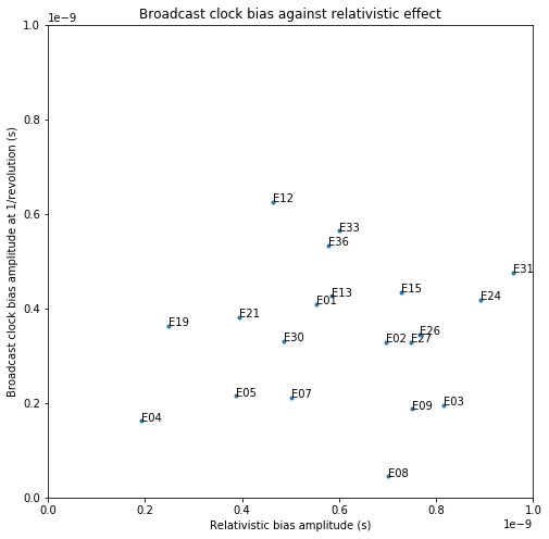
The complex amplitudes \(\alpha_{\mathrm{bias}}\) and \(\alpha_{\mathrm{drift}}\) are computed as defined above for each Galileo satellite using the broadcast ephemerides transmitted during November. To eliminate long-term effects, a polynomial of degree 4 is fitted and removed from the clock bias time series, and the average of the clock drift time series is also removed. The figure below compares the amplitude \(|\alpha_{\mathrm{bias}}|\) with the amplitude of the relativistic clock bias term for each of the satellites.
Next we compare the \(|\alpha_{\mathrm{drift}}|\) with the amplitude of the relativistic clock drift term.
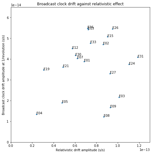
Additionally, E14 and E18, which do not appear in these graphs, have a very large relativistic amplitude, while the amplitude of their broadcast clock oscillations is similar to that of the other satellites. This was first observed by Bert Hubert.
Therefore, there is no apparent correlation between the relativistic term and the amplitudes of the oscillations of the broadcast clocks. It seems that these oscillations are not related to relativistic effects, or to any other factor depending exclusively on the eccentricity of the orbit.
Since the derivative of \(e^{in_0t}\) is \(in_0e^{in_0t}\) and the clock drift term is supposed to be the derivative of the clock bias term, we expect that \(in_0\alpha_{\mathrm{bias}}\) and \(\alpha_{\mathrm{drift}}\) are similar. The figure below compares \(n_0|\alpha_{\mathrm{bias}}|\) and \(|\alpha_{\mathrm{drift}}|\).
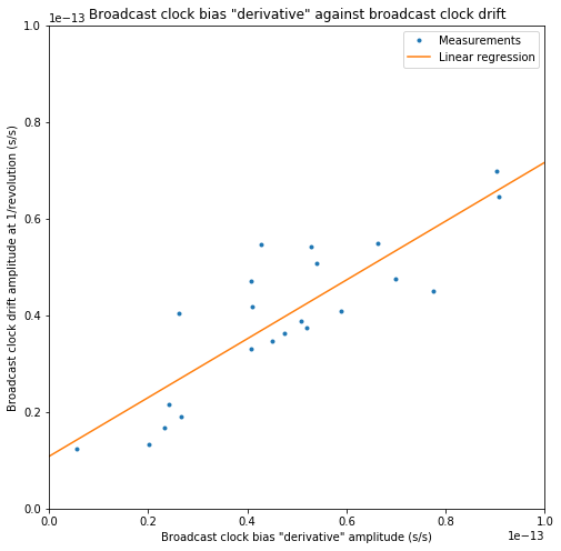
A linear regression is also shown. The slope is 0.6, and the correlation coefficient is 0.85. This is somewhat strange, as we would have expected a slope of one.
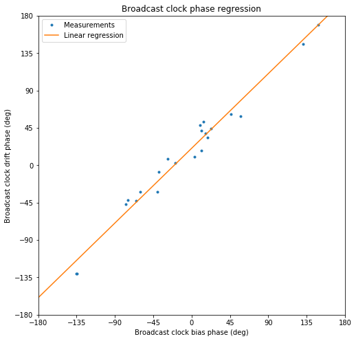
Next we compare the phases (complex arguments) of \(\alpha_{\mathrm{bias}}\) and \(\alpha_{\mathrm{drift}}\). In order to obtain a clearer graph, we plot the arguments of \(-\alpha_{\mathrm{bias}}\) and \(-\alpha_{\mathrm{drift}}\) instead (which just corresponds to adding 180º to the argument).
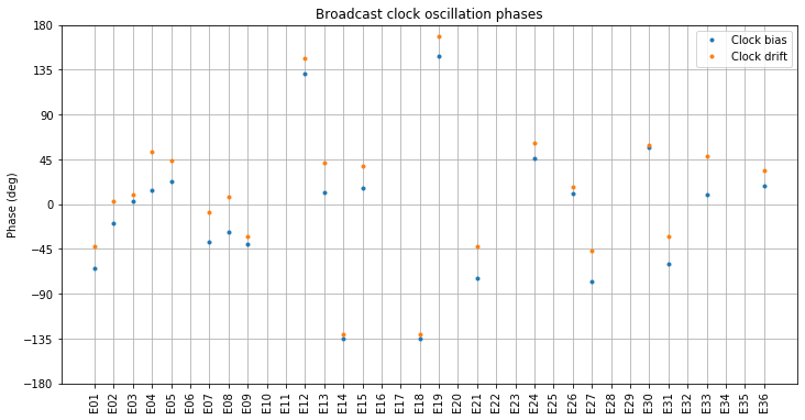
Two things are noteworthy in this figure. First, the difference between the phases of the clock bias and the clock drift is small. Since the clock drift is supposed to be the derivative of the clock bias, we would have expected a phase difference of 90º, so this is rather striking.
Additionally, the phase of most of the satellites is around 0º. Since the orbital radius is proportional to \(1-\varepsilon \cos E\), where \(\varepsilon\) denotes the eccentricity, and we are plotting the phase of \(-\alpha\), a phase close to 0º means that there is a positive correlation between orbital radius and clock bias and drift. As the radius grows, the clock bias and drift both grow.
The figure below shows a linear regression for the phase of the broadcast clock drift in terms of the phase of the broadcast clock bias. The slope is close to one, and the phase difference is approximately -20.4º, with a standard deviation of 11.5º.
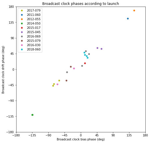
While most of the phases of the broadcast clocks are around zero, there are some outliers. The phases of eccentric E14 and E18 are close to -135º. The other outliers are E12 and E19, with phases between 135º and 180º. These satellites are the IOV satellites (recall that the E11, the other active IOV satellite) was not studied since it was unavailable during most of November.
The FOC satellites in quasi-circular orbits have phases around 0º. There is a certain correlation between the phase and in what launch each satellite was put in orbit. The figure below shows the satellites coloured by launch. We see that launches 2015-045, 2017-079 and 2018-060 cluster rather tightly. However, launches 2015-079, 2016-030 and 2016-069 do not cluster so well.
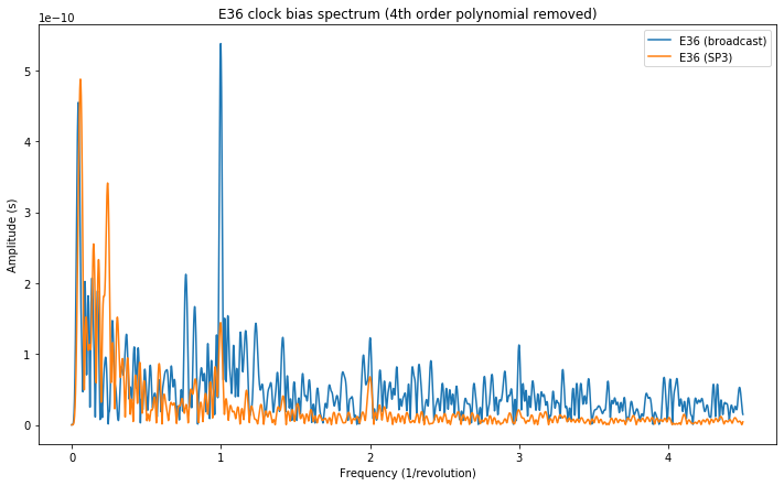
Finally, I have also plotted the spectra of the broadcast and SP3 clock biases and broadcast clock drifts of all the Galileo satellites. The list of all the plots can be found at the end of this Jupyter notebook. We see that the frequency component at 1/revolution is clearly visible in most of the plots of the broadcast clock bias and broadcast clock drift.
Some of the satellites, such as E36 shown below display a noticeable frequency component at 1/revolution in the SP3 clock. This is most likely due to clock contamination from inadequate orbit modelling. However, the component in the broadcast clock is always much larger.
So far it seems that any possible relativistic causes for these broadcast clock oscillations have been ruled out. The most likely case for these oscillations now seems unmodelled effects in the orbit solution contaminating the clock solution, as some people have already suggested.
If this is the case, then these results would indicate that the modelling done by the orbit determination centres that produce the SP3 orbits and clocks is better than the modelling done by the centre computing the broadcast orbits and clocks. Of course this is not a very fair comparison, since the SP3 final solutions are provided after one week, while the broadcast ephemerides are computed in advance.
Additionally, for the sake of fair comparisons it is convenient to mention that it is somewhat more difficult to model the orbits of Galileo satellites in comparison to other GNSS satellites, such as GPS satellites, since the Galileo satellites have a higher cross-section to mass ratio that causes larger solar radiation effects. Also, the cross-section of a Galileo satellite varies noticeably with the orientation, because the body of the satellite is elongated. This means that other GNSS constellations might not display these oscillations in their broadcast clocks simply because their orbit modelling is easier, and not because the models or algorithms used for Galileo are any worse.
In any case, these considerations are at best ramblings without more data supporting the hypothesis that the cause of the oscillations is inadequate orbit modelling. Some of the additional questions that this post raises are why the clock bias and clock drift oscillations do not have the amplitude and phase relationship that one would expect in a derivative, and why there seems to be some kind or correlation between the satellite type (recall that the IOV and FOC satellites are physically very different) and launch, and the phase of the oscillations.