On April 28, I got together with a few Spanish radio Amateurs to perform some experiments. One of the things we did was an angle of arrival experiment in the 145MHz Amateur band. The ultimate goal of the experiment was to be able to measure the angle of arrival of meteor reflections of the GRAVES radar at 143.05MHz. However, we also recorded a few other signals, such as the Amateur satellite band at 145.9MHz (intended to perform calibration of the setup) and the APRS terrestrial signals at 144.8MHz.
The antennas used in the experiment can be seen in the figure below. They are a pair of J-pole antennas built with copper pipe. The supports are PVC pipes. The antenna spacing is 1/2 wavelength at 143.05MHz. A run of around 15m of 75 Ohm TV coaxial cable is used to connect each antenna to the receiver.
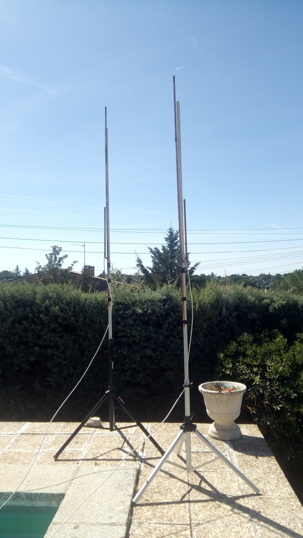
This setup is less than ideal. The J-pole antennas were quickly built for the experiment, their impedance wasn’t measured, and using 75 Ohm coax is not optimal. However, they worked fine for strong signals. Also, the receiving location is not ideal. As it can be seen in the image, it is a suburban location with low buildings, so many of the signals arrive with multipath or in a non-line-of-sight manner.
The receiver is a LimeSDR. Its two channels are used to receive coherently from both antennas, so that the phase difference of the signals can be measured easily, in order to determine the angle of arrival. The spacing of 1/2 wavelength for the antennas was chosen to prevent the phase ambiguities that appear with a larger spacing.
The antenna baseline was laid so that the line perpendicular to the baseline had an orientation of approximately 35º. The antenna due northwest (right antenna in the figure above) was connected to the first channel of the LimeSDR, while the antenna due southeast was connected to the second channel.
The LimeSDR was set to a centre frequency of 145MHz and a sample rate of 5MHz. The LNAL input was used for both antennas, with an LNA gain of 30dB, TIA gain of 12dB, and PGA of 0dB. In order to save disk space, the following sub-bands of the full 5MHz of bandwidth were selected and recorded as IQ samples using 32bit floats:
- APRS: 144.800MHz, 25ksps
- GRAVES: 143.050MHz, 5ksps
- Satellites: 145.900MHz, 250ksps
The recording was made with the following GNU Radio flowgraph. The time span of the recording was from 09:48:40 UTC to 10:52:30 UTC. The recording files can be found here, together with a description of the recording format.
Satellites
The main interest of recording the 145MHz Amateur satellite band was to have a means of calibrating the setup and being able to determine the phase difference caused by the difference in feed line length to each antenna, as well as obtaining a more precise measurement of the antenna separation and the baseline orientation.
In theory, since the angle of arrival of a satellite signal can be computed from its TLE parameters, it is possible to compare this calculation with the measurements in order to determine the unknown parameters of the antenna array. An ideal signal for this is a line-of-sight signal that sweeps a large range of angles of arrival, so low Earth orbit satellite passes can be used as calibrators.
The satellite Nayif-1, which had a pass at 10:09 UTC was an ideal opportunity, since it transmits continuously a 1k2 BPSK telemetry signal at 145.940MHz.
This GNU Radio flowgraph was used to filter 10kHz of spectrum centred at 145.940MHz and to separate both channels for easier processing. The signal is then cross-correlated and analyzed in the following Jupyter notebook.
The position of Nayif-1 in the sky can be seen in the figure below. The azimuth sweeps a large range of angles of arrival, but unfortunately the elevation is not very high. This, together with the terrain obstructions around the antennas gave problems with multipath and non-line-of-sight signals, as we will see.

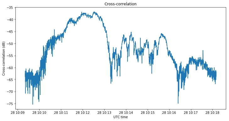
The magnitude of the cross-correlation is seen below. A coherent integration period of 100ms has been used in the correlation. The noise floor is seen in the left part of the graph to be at around -63dB. In the first minutes of the pass the signal is quite good, reaching up to 25dB SNR in cross-correlation. However, after 10:13, the signal presents deep fading typical of a Rayleigh channel.
The next figure shows the signal power received in each of the antennas. The power measured by antenna 2 has been increased by 5dB in the plot, because for some unknown reason the second channel showed less signal level than the first channel. We can see that the power at each antenna follows a different pattern, especially after 10:13 UTC. This is spatial diversity, which indicates multipath caused by nearby objects.

The figure below shows the comparison between the measured and the theoretical phase difference between each of the channels. The theoretical value has been obtained from the azimuth and elevation shown above, assuming a baseline orientation of 35º and length of 1/2 wavelength, and it has been adjusted vertically by hand to compensate for the phase difference between channels due to the difference in feed lines.
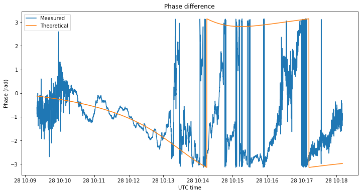
We can see that between 10:10 and 10:13 the measurements track approximately the theoretical value, although large excursions can be seen. This means that the signal is arriving with a certain degree of multipath rather than in a pure line-of-sight manner. After 10:13, the measurements no longer resemble the theoretical value at all, indicating that the signal is now arriving completely by non-line-of-sight.
Unfortunately, the multipath effects in the observation of Nayif-1 make it impossible to use this measurements to calibrate the antenna array.
APRS
In the recording there are APRS signals from several terrestrial stations. However, only the signals from ED4ZAE-3 are strong enough to be decoded. I wasn’t able to decode the signals from the remaining stations using Direwolf, so I don’t know their locations.
The calibration information about the phase difference due to different feedlines cannot be easily translated from 145.94MHz to 144.8MHz, so a new calibration has been made for APRS. Assuming a baseline orientation of 35º and length of 1/2 wavelength as above, the phase difference has been calibrated taking into account that the signals from ED4ZAE-3 should arrive from 237º, which is the straight line direction to the station. Note that this is only an approximate calibration. The phase difference of the signals from ED4ZAE-3 varies around 10º due to multipath propagation.
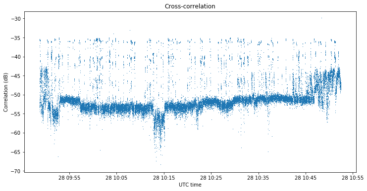
The figure below shows the cross-correlation magnitude in dB. The noise floor is between -55dB and -50dB, due to varying levels of interference. We have signals as strong as -35dB. As above, the coherent integration period for the correlation is 100ms.
Below we show the angle measurements obtained for signals stronger than -41dB (this is made to filter out time intervals where no APRS packet was transmitted). The angle is shown as a relative angle to the baseline direction (35º). Therefore, an angle of -20º corresponds to an azimuth of 15º or 235º. Note that the radiation pattern for a phased array consisting of only two antennas is always symmetric with respect to the baseline, so such an array is unable to distinguish between angles of arrival which are symmetric with respect to the baseline.
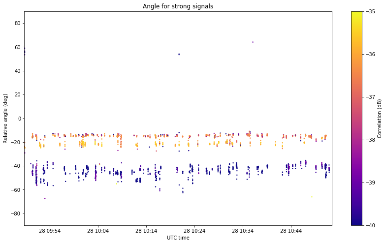
The strength of the signals is color-coded as shown on the right of the graph. We see that the strongest signals, in yellow, which correspond to ED4ZAE-4, arrive from a relative angle of around -22º, as marked by the calibration. There is another station at around -15º which is slightly weaker than ED4ZAE-4, and some other station or stations between -40º and -50º. In this last case, the signals are weaker and the angles of arrival vary much more, probably due to greater multipath. It is also interesting to note that all the signals arrive from a relatively small interval of directions between -60º and -10º.
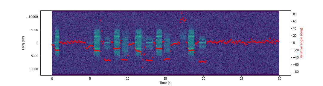
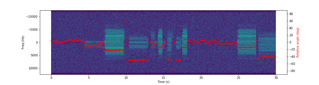
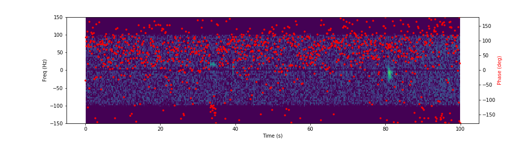
The two figures below show a couple of small excerpts from the recording. The spectrum is shown to aid identifying the different stations by their different strength and different modulation pattern (most likely caused by different FM deviations). The angle of arrival is shown using red dots. It is interesting to see how the different stations can be identified according to their angle of arrival. It is also interesting to note that the noise floor comes mostly from a well defined direction.
The analysis of APRS signals has been done in this Jupyter notebook.
GRAVES
In the case of meteor scatter pings from GRAVES, the results are not very good. The recording has been filtered down to 200Hz of bandwidth and 1ksps using this GNU Radio flowgraph. The same kind of plot as for the APRS signals has been done, but without calibrating the phase offset, so the measures are phase differences instead of angles of arrival. This was done in the following Jupyter notebook.
Some of the most interesting excerpts from the recording are shown below. In comparison to the APRS excerpts shown above, the noise floor doesn’t come from any specific direction, as is to be expected if there is no noticeable interference.
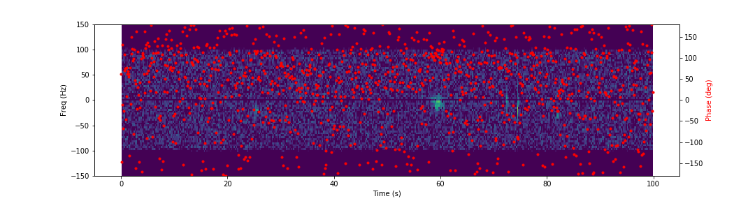
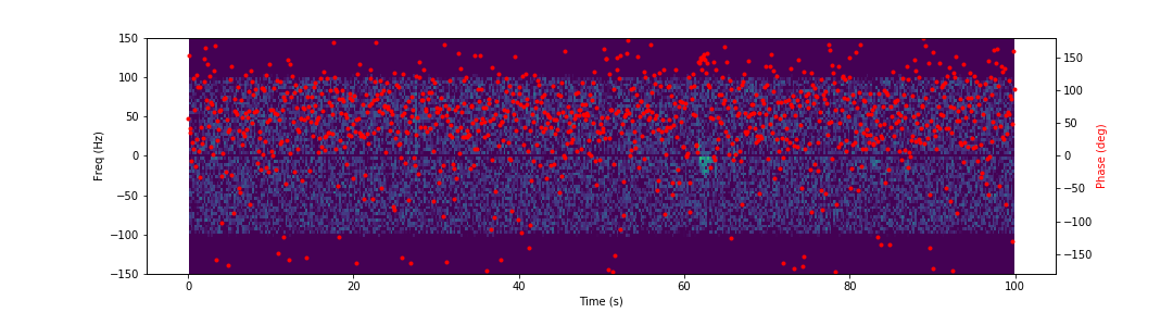
Only the strongest and longest meteor scatter bursts produce phase difference measurements that are distinguishable from background noise, and even so, the quality of these measurements is not so good. Moreover, the phase differences corresponding to different bursts are completely different. This may be caused by the signals arriving by heavy multipath because of obstacles in the direction to GRAVES.
The array baseline was oriented perpendicularly towards GRAVES, so as to give the best sensitivity in measuring angles from the direction of GRAVES. However, that direction was blocked by low houses.
From the analysis of these results, it seems that to measure the angle of arrival of GRAVES pings successfully it is very important to have a clear view to the horizon. Also, using small yagis instead of omnidirectional antennas might help. If an observation using a baseline of 1/2 wavelengths such as in this experiment is able to determine that the angles of arrivals of GRAVES pings are all confined to a small range of azimuths, it is recommended to perform a second observation using a longer baseline, so as to obtain a greater sensitivity in the determination of the angles of arrival.
I would like to thank Luis Bernal EA5IDN, Gonzalo Carracedo EA1IYR, and Esteban Dauksis for their great help in the preparation and performance of this experiment.
really interesting. Well written.
Hello!
I was interested in your experiment on coherent signal reception using the LimeSDR-USB. I tried to run your GNU Radio flowgraph (limesdr_2m_aoa.grc), but I got an error in the limesdr_rx_source, linrad_server, linrad_send_raw16 blocks. Where can I get the missing modules?
Hi Alexander, the limesdr_rx_source block can be found here (copy the file to
~/.grc_gnuradio/), while the Linrad blocks come from gr-linrad.Thank you. It all worked.
Unlike LimeSuite_Source GRC-blok in limesdr_rx_source, it is possible to set its own frequency for each channel. At the same time, the frequency difference between the channels should not exceed 30.72 MHz, right?
Hi Alexander. Both channels share the same LO. You could “tune” to different frequencies by using the NCO. The tuning limit using this method is (in theory) plus-minus one half of the ADC rate.
Dear Daniel Estevez
What is the accuracy of AOA estimation using your method?
Hi John,
In this experiment it is hard to tell what the accuracy was, since the calibration with Nayif-1 was a complete disaster. Theoretically, assuming that everything is calibrated correctly, an angular resolution comparable to a fraction of the inverse of the baseline length in wavelengths can be achieved. However, calibration is important and difficult in many cases, so it will place a limit to the performance often.
Dear Daniel Estevez
I tried to run your GNU Radio flowgraph (limesdr_2m_aoa.grc) with hardware LimeSDR-USB, but I got the following error error, how to due with it?
Loading: “C:\Users\admin\Desktop\gnu\limesdr_2m_aoa.grc”
>>> Done
Generating: ‘C:\\Users\\admin\\Desktop\\gnu\\limesdr_2m_aoa.py’
>>> Warning: This flow graph may not have flow control: no audio or RF hardware blocks found. Add a Misc->Throttle block to your flow graph to avoid CPU congestion.
Executing: C:\Python27\python.exe -u C:\Users\admin\Desktop\gnu\limesdr_2m_aoa.py
/home/daniel/aoa_aprs_2019-09-24T08:31:58.748000.2xc64: Invalid argument
Traceback (most recent call last):
File “C:\Users\admin\Desktop\gnu\limesdr_2m_aoa.py”, line 257, in
main()
File “C:\Users\admin\Desktop\gnu\limesdr_2m_aoa.py”, line 245, in main
tb = top_block_cls()
File “C:\Users\admin\Desktop\gnu\limesdr_2m_aoa.py”, line 136, in __init__
self.blocks_file_sink_0_0_0_0 = blocks.file_sink(gr.sizeof_gr_complex*1, filename_aprs, False)
File “C:\Program Files\PothosSDR\lib\python2.7\site-packages\gnuradio\blocks\blocks_swig0.py”, line 509, in make
return _blocks_swig0.file_sink_make(itemsize, filename, append)
RuntimeError: can’t open file
You don’t have the /home/daniel/aoa_aprs_2019-09-24T08:31:58.748000.2xc64 file. Please set the path of this file in the flowgraph to the correct path where this file is stored in your system.
thanks for your apply, I solved this problem with your help,but I come with new problem: self.linrad_send_raw16_0 = linrad.send_raw16(“127.0.0.1”, 50000, freq * 1e-6, 0x1000)
AttributeError: ‘module’ object has no attribute ‘send_raw16’,
from https://github.com/daniestevez/gr-linrad/, I have download gr-linrad and compile install it, from http://www.sm5bsz.com/linuxdsp/linrad.htm, I also have download linrad and compile install it, I can configure linrad gui parameters successfully, but in grc it doesn’t work, with no attribute ‘send_raw16’ or ‘send_raw24’, can you give me some help, thanks!
Do you have swig installed? Did gr-linrad compile successfully? Did you run ldconfig as root after installing gr-linrad?