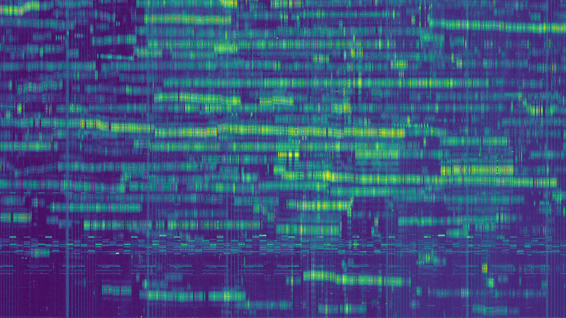
Last weekend, I recorded the full EAPSK63 contest in the 40m band with the goal of monitoring IMD levels. I made a 48kHz IQ recording spanning the full 24 contest hours (from 16:00 UTC on Saturday to 16:00 UTC on Sunday). This week I’ve been playing with making waterfall plots from the recording. These are very interesting, showing patterns in propagation and contest activity. Here I show some of the waterfalls I’ve obtained, together with the Python code used to compute them.
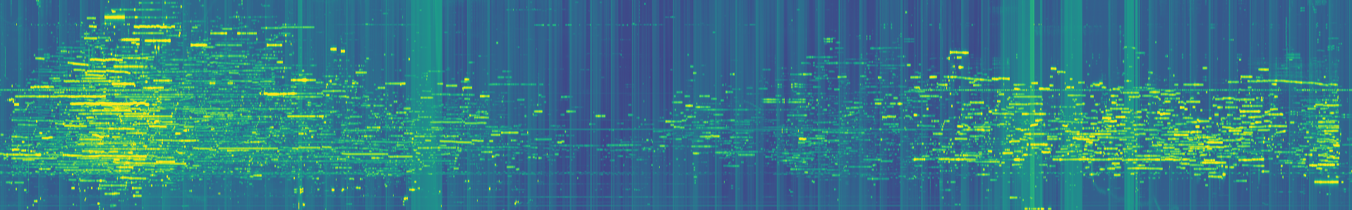
In all the waterfalls shown here, time is represented in the horizontal axis, and frequency is represented in the vertical axis, with the top of the image corresponding to the highest frequency and the bottom of the image corresponding to the lowest frequency. All the plots are done with FFT transforms overlapping a 50% and the Blackmann window. The banner on top of this post is cropped from a waterfall done with 1024 FFT bins and 4308 averages, thus producing a 1920×1024 image. The resolution is 46.86Hz or 49.96s per pixel.
The image below shows a comparison between the JT65 and JT9 activity and the EAPSK63 contest. It is cropped from a waterfall with 4096 FFT bins and 1077 averages, yielding a 1920×4096 image with a resolution of 11.72Hz or 45.99s per pixel. Remember that you can click on the images to view them in full size.
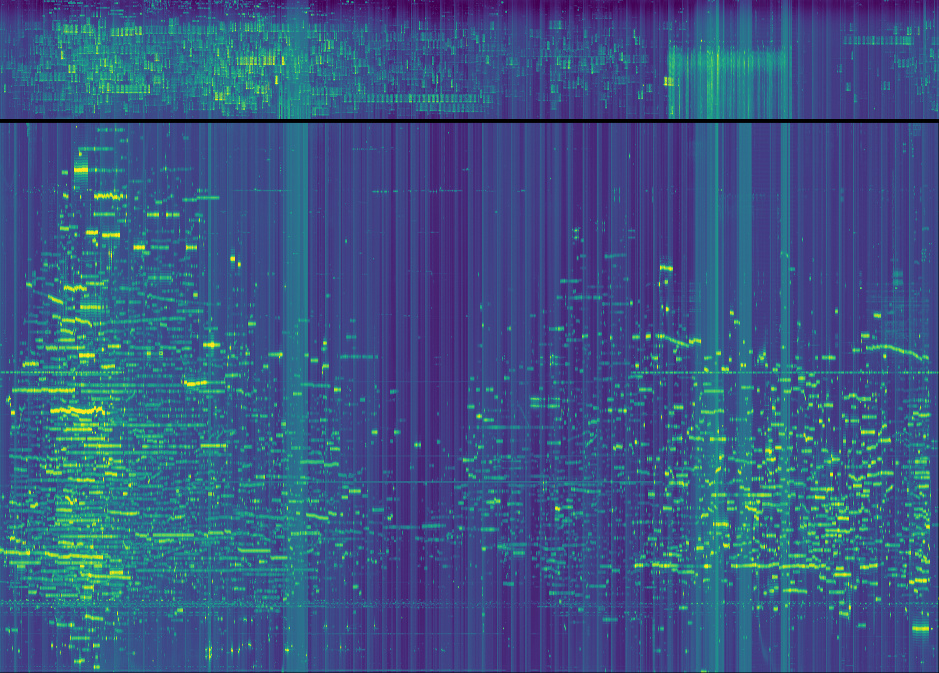
A large number of the stations participating in the EAPSK63 contest are located in Spain. Hence, their signal is usually strong at my station in Madrid, but late at night this time of the year Spain is in the skip zone for 40m, so Spanish stations are weak or not present at all. Thus, at night only stations elsewhere in Europe and outside Europe are present. The proportions of local and DX stations in the PSK contest and in JT modes are quite different. Also, the patterns of activity throughout the day are different. The JT modes activity depends basically on propagation (people choosing the best bands trying to work DX), while the contest activity has much to do with the local time in Europe. Therefore, we can see really different patterns in the waterfall.
On Saturday night, the JT activity is at its peak, while the contest activity has diminished and is almost non-existent late at night. On Sunday noon, there is strong contest activity, but the JT segment is almost clean and sometimes occupied by SSB stations, since propagation in 40m is too short for DX during the day. The WSPR segment can also be seen near the bottom of the image above. WSRP signals depend almost exclusively on propagation, as activity is roughly constant. However, it is a bit difficult to judge the strength and number of WSPR signals in this waterfall.
The image above was cropped from the following 1920×4096 image. A portion of this image can be cropped to obtain a 1920×1080 image, which can be used as a desktop background.

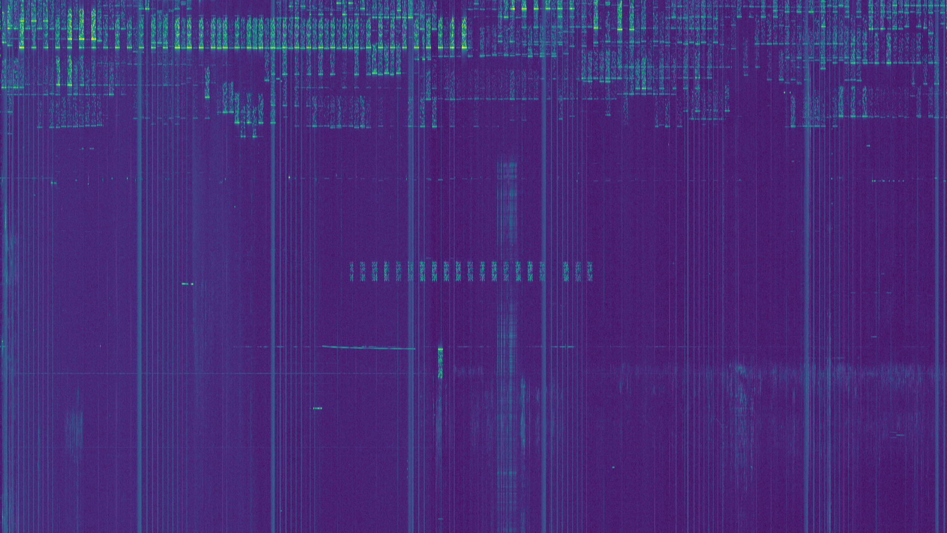
I have also done a high resolution waterfall with 16384 FFT bins and 29 averages, which yields a 17830×16384 image with a resolution of 2.93Hz or 5.12s per pixel. In this large image, I’ve found the following interesting regions. All of them are 1920×1080 crops. They are best viewed in full size.
Lots of activity in JT65 and JT9.

A station calling CQ in QRA64A. Unfortunately, no takers. You can also see a JT65 station using the wrong sideband (LSB).
Some stations doing DSSTV using HamDRM, which uses LSB on 40m.
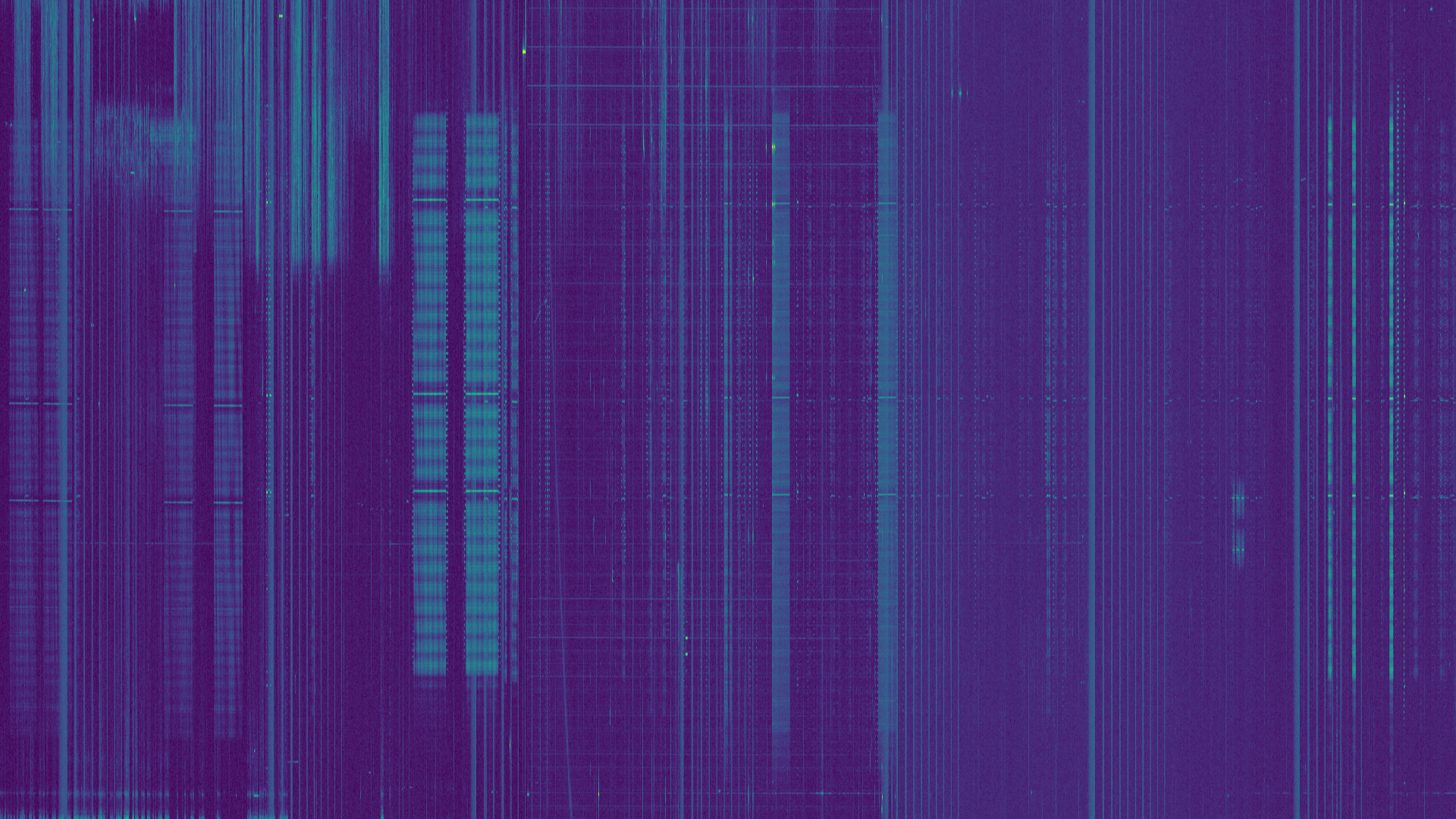
The WSPR segment and the EAPSK63 contest fray, with PSK stations transmitting sometimes on top of the WSPR segment or below 7040kHz.
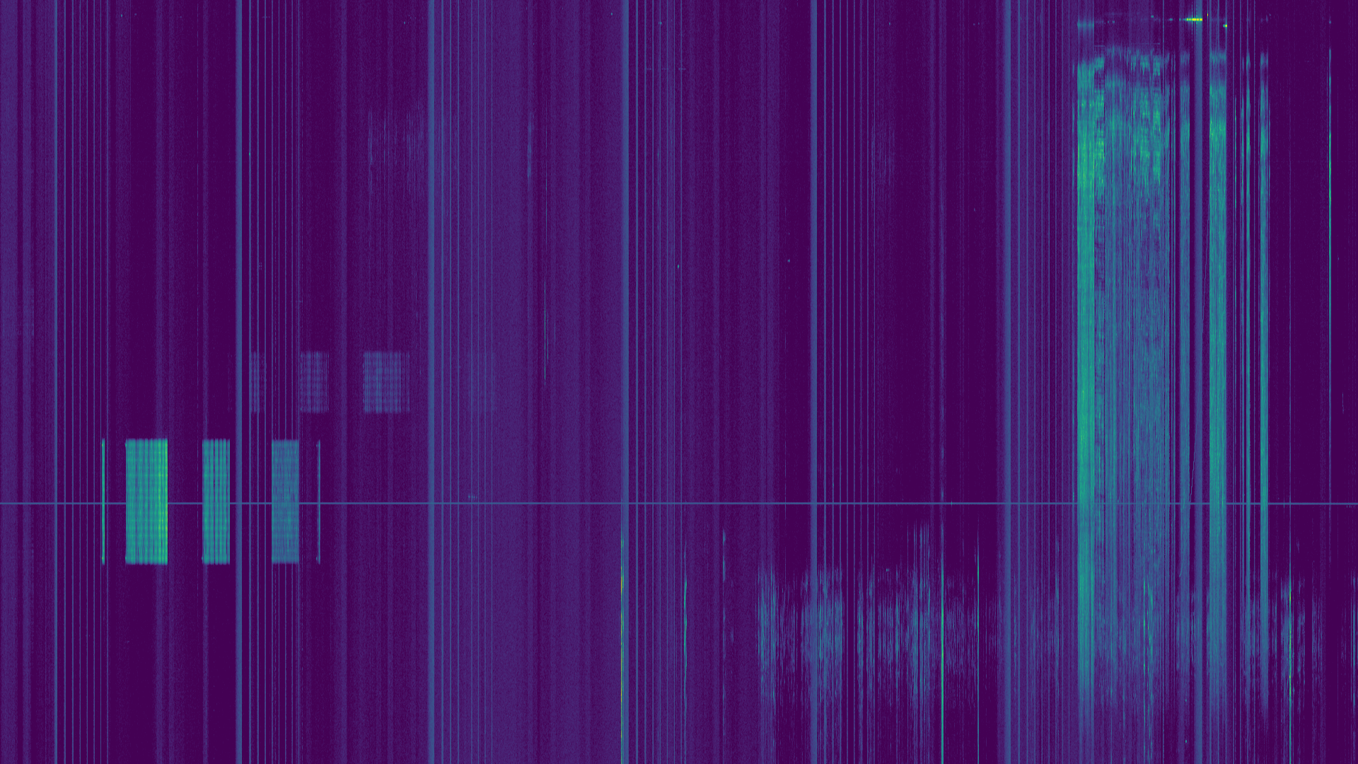
Two stations using some kind of MFSK digital modes and an SSB station.
The code used to plot the waterfalls in this post is as follows:
This code can be adapted to process any other recordings or for experimenting with different parameters and the EAPSK63 contest recording (perhaps different FFT windows can be tried). It saves the averaged transforms in a file, so computation can be stopped midway and resumed later on or plotting parameters can be changed without having to recompute the FFTs. The waterfall is plotted in PNG chunks to prevent the plotter from running out of RAM. The chunks can be merged later with Imagemagick by doing
convert +append waterfall?.png waterfall.png
One comment