This is a follow up post to my experiments studying OTH radar. I have found that the signal processing I did there to obtain the cross-correlation was far from optimal. This produced the strange side-bands below the main reflection. The keen reader might have noticed that I was doing the cross-correlation with a template pulse that lasted the whole pulse repetition cycle. However, the pulses from the radar are shorter. Therefore, it is a better idea to use a shorter template pulse. Ideally, the template pulse should have the same length as the transmitted pulse. However, I don’t know this length precisely, because multipath propagation makes the received pulses a bit longer. However, I think that 6.5ms is a good estimate.
I have also changed the window for the pulse. I’m now using a Dolph-Chebyshev window. I use scipy to compute this window, because it is not included in GNU Radio. This window has the property that the side-bands have constant attenuation. Indeed, it minimizes the \(L^\infty\) norm of the side-bands. There is a parameter that tunes the side-bands attenuation. For higher attenuations, you have a wider main lobe, while if you want a narrower main love you get less side-band attenuation. These properties make this window useful in radar applications.
Below I’m doing the cross-correlation in GNU Radio with a shorter template pulse shaped with a Dolph-Chebyshev window set for 55dB attenuation.

The good thing about the settable attenuation of the Dolph-Chebyshev window is that it can be used to trade-off performance between different features. First, we use an attenuation of 100dB. The side-bands are below the noise floor in this case, so we have no “false responses” in our cross-correlation. The drawback is that the main lobe is wide so the resolution of the features of the ionosphere in the image below is not very good.

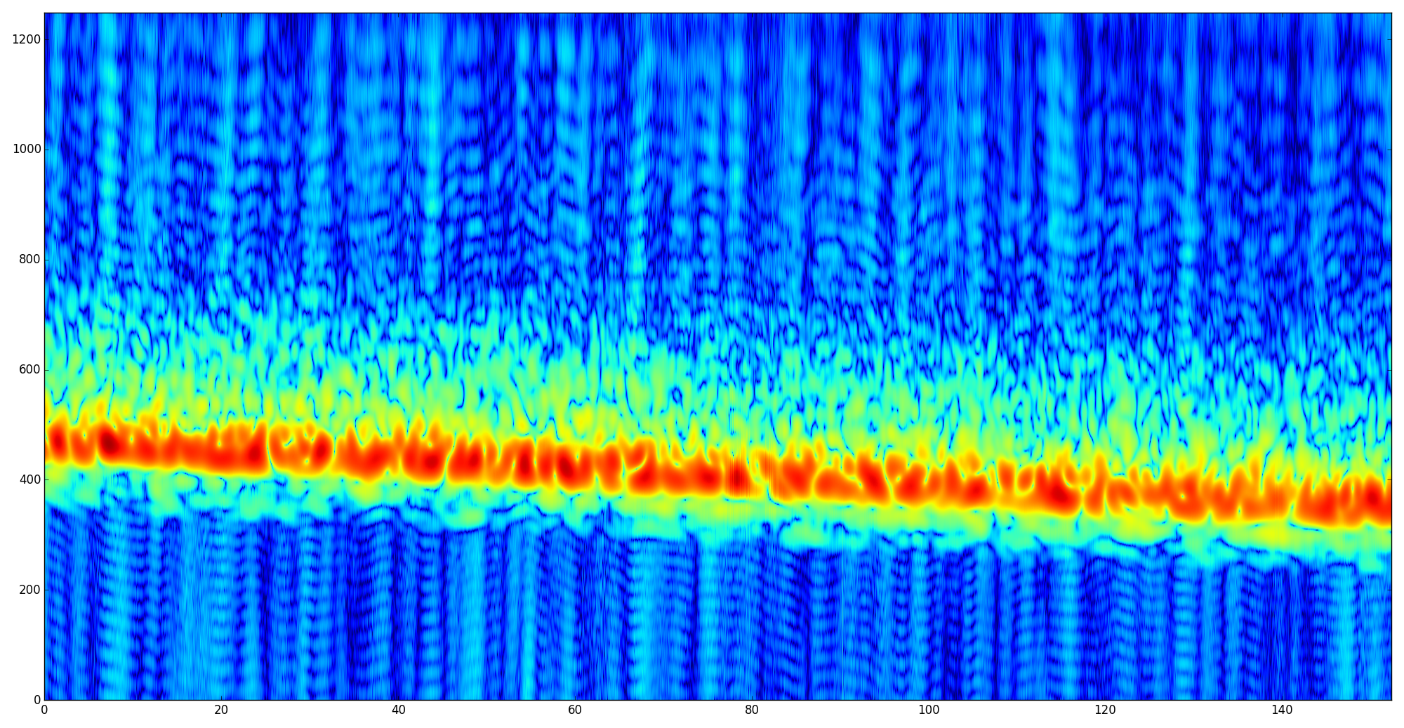
Next we try with 55dB attenuation. This narrows the main lobe, improving the resolution and crispness of the features of the ionosphere in the image below. However, side-bands start being visible above the noise floor, producing “false responses”. However, comparing with the image above, we now know where the false responses are.
I have updated the gist with the GNU Radio flowgraph and python script used to produce the images.
One comment