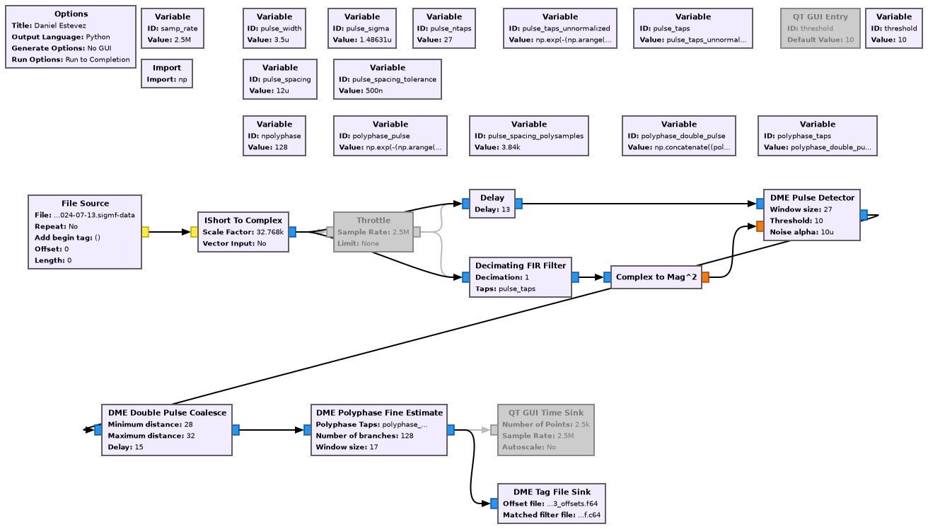
You might remember that back in July I made a recording of the DME ground-to-air and air-to-ground frequencies for a nearby VOR-DME station. In that post, I performed a preliminary analysis of the recording. I mentioned that I was interested in measuring the delay between the signals received directly from the aircraft and the ground transponder replies, and match these to the aircraft trajectories. This post is focused on that kind of study. I will present a GNU Radio out-of-tree module gr-dme that I have written to detect and measure DME pulses, and show a Jupyter notebook where I match aircraft pulses with their corresponding ground transponder replies and compare the delays to those calculated from the aircraft positions given in ADS-B data.
GNU Radio DME receiver: gr-dme
I have written a new GNU Radio out-of-tree module called gr-dme to detect and measure DME signals. This OOT module includes several blocks that work in tandem to annotate an IQ stream with tags that mark the location of DME pulse pairs, as well as their complex amplitude and fine (subsample) time estimate. A block called DME Tag File Sink writes the data in these tags into binary files, but the tags can also be used to trigger a QT GUI Time Sink for real time visualization of the DME pulses, or for further processing in GNU Radio.
The following figure shows the flowgraph I have used to measure the DME pulse pairs from my recordings. Each of the custom blocks is explained below.
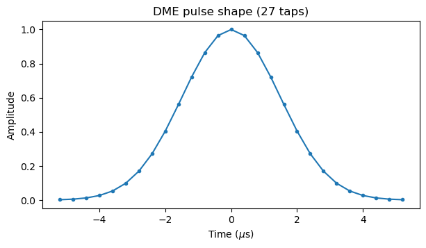
The IQ data in the recording is sampled at 2.5 Msps. The first step in the processing is to pass the IQ data through a matched filter for a single DME pulse. Therefore, the first question is how to model the DME pulse shape. I haven’t found an exact description of the DME pulse shape. It appears to be specified only in terms of parameters such as pulse width, rise time and fall time, and the exact shape probably varies slightly with each equipment (which might give a way to fingerprint equipment). I found a Performance specification Distance Measurement Equipment (DME) transponder system document from the FAA that has been quite useful. It mentions that the transponder output signals have a pulse width of 3.5 ± 0.5 μs, and a rise and decay time of 2.5 +0.5/-1.0 μs. The pulse width is measured between the 50% amplitude points of the leading and trailing edge of the pulse, and the rise and decay times are measured between the 10% and 90% amplitude points. This application note from Rohde & Schwarz is also a useful reference.
I have decided to model the DME pulse as a Gaussian\[\frac{1}{\sqrt{2\pi\sigma^2}}e^{-\frac{x^2}{2\sigma^2}}.\]Since the pulse width \(W\) is defined as the distance between the 50% amplitude points, the standard deviation parameter \(\sigma\) for the Gaussian can be calculated as\[\sigma = \frac{W}{2 \sqrt{2 \log 2}}.\]The rise and decay times of this Gaussian measured between the 10% and 90% levels are then\[\frac{W}{2}\left(\sqrt{-\frac{\log 0.1}{\log 2}} – \sqrt{-\frac{\log 0.9}{\log 2}}\right).\]For \(W = 3.5\) μs this gives 2.507 μs, so it matches quite well the specification.
I have used 27 taps for the DME pulse shape at 2.5 Msps. The value of the first and last tap is 0.002, so using more taps isn’t necessary. The taps of this matched filter are shown here.
The IQ signal is filtered with this matched filter and the power is computed with the Complex to Mag^2 block. The original IQ signal also passes through a Delay block that introduces the same delay as this matched filter, in order to preserve the alignment between the two signals. These two signals go into the DME Pulse Detector block. The goal of this block is to detect the presence of DME pulses according to the power of the matched filter, and to add a tag marking the approximate location of the peak of each pulse.
The DME Pulse Detector block keeps a running estimate of the noise floor level by passing the matched filter power through a one-pole IIR filter with a long time constant. Since the duty cycle of the DME pulses is low, the positive bias they introduce in this estimate is small. Whenever the matched filter power gets above the noise floor estimate multiplied by a threshold, a detection is declared. The block then looks forward in a window of \(N\) samples to find the maximum matched filter power in this window. The location of the maximum is taken as the pulse peak location and a pulse tag is added to the corresponding sample in the IQ stream. The block doesn’t produce any more pulse detections within this window. The window length \(N\) is set equal to the matched filter length. The output of this block looks like this on a QT GUI Time Sink
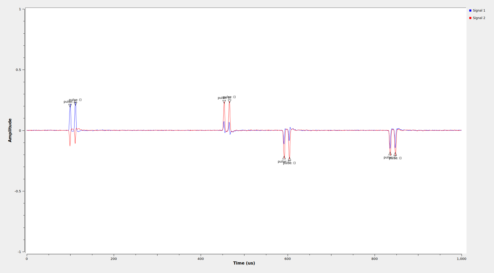
The next block is the DME Double Pulse Coalesce. The goal of the block is to convert detections of individual pulses into detections of pulse pairs, with a single pulse tag in the middle of the pair. The block works only with tags, and doesn’t look at the values of the IQ samples. Whenever it sees a pulse tag, it looks ahead in a window defined by the minimum distance and maximum distance parameters (which are defined in terms of the DME pulse spacing). If a second pulse tag is found inside this window, then an output pulse tag is added at the location of the first pulse tag plus a certain delay (also defined by the DME pulse spacing). If a second pulse tag is not found, then an output pulse tag is not emitted, effectively discarding this detection. Note that the detection of pulse pairs done by gr-dme doesn’t look at the gap between pulses and require a low amplitude there, which is something that a better DME receiver might do to try to reject interference. In particular, a long pulse which encompasses the whole duration of the DME pulse pair will trigger the gr-dme detection successfully. The output of this block looks like this.
Finally, now that DME pulse pairs have been detected and the coarse location of their midpoint has been found, the DME Polyphase Fine Estimate performs an accurate measurement of the pulse pairs to determine their timestamp (including sub-sample delay) and complex amplitude. As it name indicates, it does so by filtering the IQ signal with a polyphase filterbank that contains a matched filter for the DME pulse pair.
The polyphase filter has 128 branches, corresponding to 128 interpolation phases between each pair of consecutive 2.5 Msps IQ samples. This gives a time resolution of 3.125 ns, which is roughly one metre, more that adequate for this application. The prototype filter is shown in this plot.
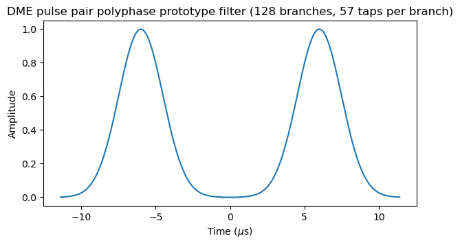
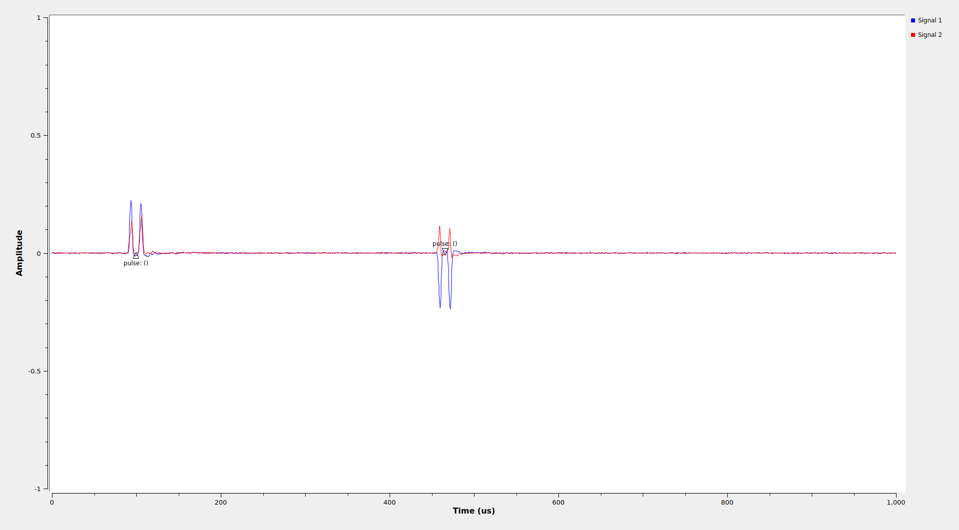
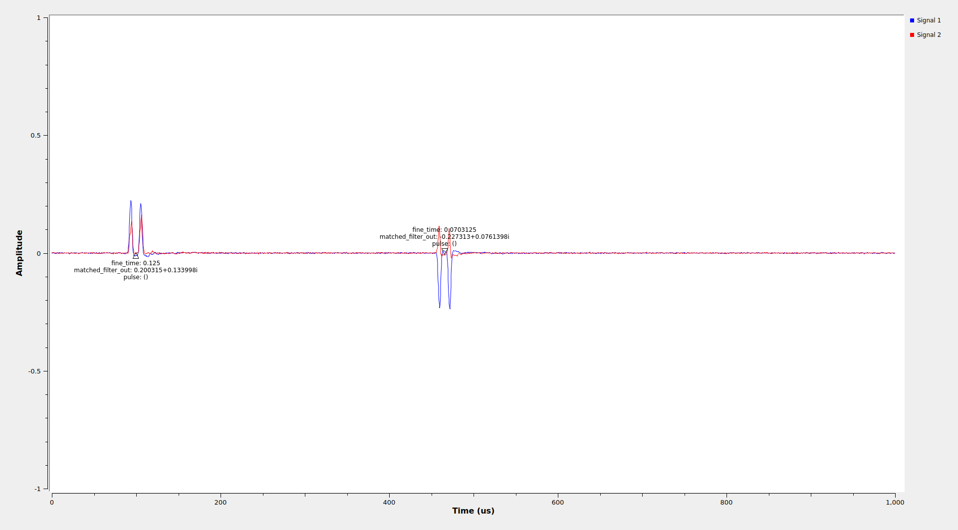
When the DME Polyphase Fine Estimate block sees a pulse tag, it computes the matched filter output for all the 128 branches of the polyphase filterbank and for integer sample offsets in a window of \([-M, M]\) samples with respect to the location of the tag. The matched filter output that gives the highest power determines the fine time estimate of the pulse pair. This is decomposed as an integer sample time, which affects the location of the output tag, and a fractional sample time, which is determined by the phase of the polyphase filterbank that achieved the maximum and is placed in a fine_time tag at the output. The complex value of the matched filter output that attained the highest power is placed in a matched_filter_out tag. This complex value contains the pulse pair amplitude and phase. The output of this block is shown in the following QT GUI Time Sink plot.
The DME Tag File Sink block receives the output of the DME Polyphase Fine Estimate block and writes the tags to binary files. There are two files, an offsets file that contains the time offset of each pulse pair, measured in samples including the fractional part, as a float64, and the matched filter file, which includes the matched_filter_out value of each pulse pair as a complex64. This raw binary format is very compact and easy to open in NumPy, as opposed to, for instance, using SigMF annotations to store the parameters of each pulse pair.
I have run the DME receiver flowgraph using a detection threshold of 10 both for the air-to-ground and ground-to-air frequencies.
Initial analysis of DME pulse pairs
The analysis of the output of gr-dme is done in a Jupyter notebook. For each pulse pair that gr-dme has detected, we have its timestamp and its complex amplitude (measured from the matched filter output). From the complex amplitude, the main interest is the amplitude or power. The phase information is not very useful because since there are large silent gaps between pulse pairs, it isn’t possible to use the phase of the pulse pairs to estimate the frequency without ambiguities.
The recording I made had a duration of slightly over 2 hours. In this recording, gr-dme has detected 6287903 pulse pairs from the ground station and 1075427 pulse pairs from aircraft. This gives average rates of 862 and 147 pulse pairs per second respectively. These values seem reasonable. Although some sources such as this page mention that DME squitter ensures a rate of 2700 pulse pairs per second in the ground station, the Rohde & Schwarz application note says that DME squitter pulses are added to prevent the rate from dropping below 700 pulse pairs, and that TACAN squitter ensures a higher rate of 2700 pulse pairs per second (TACAN squitter pulses are also used by aircraft to measure the bearing to the ground station). Wikipedia mentions that the DME transponder has a limit of 2700 pulse pairs per second, which is reached if the transponder is used simultaneously by many aircraft. So it seems that in DME squitter is added to ensure a rate above 700 pulse pairs per second, and depending on the utilization, the actual pulse rate will be between 700 and 2700 pulse pairs per second.
Wikipedia also says that aircraft use 150 pulse pairs per second in search mode and less than 30 pulse pairs per second in track mode (ensuring an average rate not exceeding 30 pulse pairs per second when the overall usage in both modes is considered). Therefore, the value of 147 pulse pairs per second we have obtained for the air-to-ground frequency sounds reasonable, as it corresponds to an average of 4.9 aircraft. Another observation is that at low utilization rates the ground station pulse rate would be around 700 pulse pairs per second contributed by squitter plus the rate on the air-to-ground frequency (since all the aircraft interrogations are re-transmitted). In this case this almost happens. The ground station has a slightly higher rate than 700 + 147, but we have not taken into account the Morse identification, which sends pulse pairs at a rate of 1350 pulse pairs per second and so it increases this average slightly.
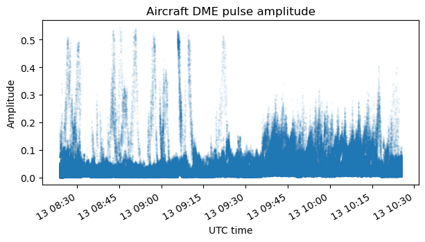
The following two plots show the amplitude or power of the ground station measured in linear amplitude units and in dB units. The power stays mostly constant throughout the recording, with small variations that can be explained by gain changes in the transmitter and receiver and slight changes in the propagation path (which was almost line-of-sight).
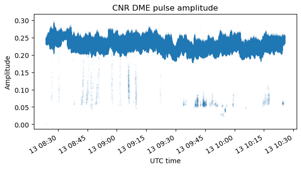
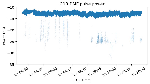
However there is something rather strange, which is that during some time intervals there are pulses which have much less amplitude than the rest. This is easily seen in the two plots above. These “small pulses” have around 10 dB less power than the rest. A zoom to a short time interval in the amplitude plot shows that really these small pulses are a minority that is transmitted occasionally.
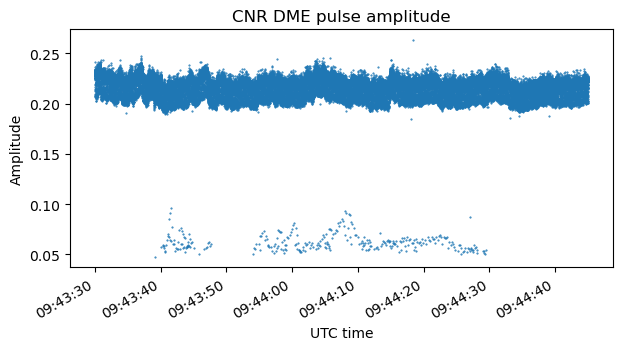
I don’t have a good idea of what causes these small pulses. I’m not even certain that they are transmitted by the ground station. They could be an artifact of my recording set up. As we will see below, the presence and power of these small pulses seems to correlate with the presence of strong signals in the air-to-ground channel. As I mentioned in the previous post, I tuned the Lime SDR to the frequency at the mid-point between the air-to-ground and ground-to-air frequencies. Perhaps this choice was not great, because any IQ imbalance would cause the IQ mirror of the air-to-ground signals to appear in the ground-to-air channel and vice versa.
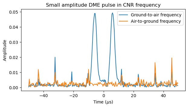
To investigate this more I have selected one of the small pulses and plotted the signal amplitude around the location of this pulse in the ground-to-air and air-to-ground channels. The small pulse detected in the ground-to-air frequency is a valid DME pulse pair, so it is not some interference that was mistaken for a DME pulse pair by gr-dme. However, we don’t see a corresponding pulse in the air-to-ground frequency. The two recordings are lined up well, judging by the fact that some pulsed interference (which is probably very wideband and affects the two channels) lines up in both channels.
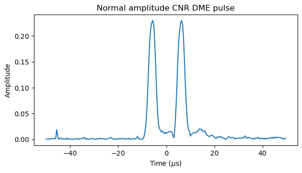
Here is a similar plot of the previous pulse pair that was found in the ground-to-air frequency. This is a normal pulse pair transmitted by the DME ground station. The normal pulse looks very similar to the small pulse, only the amplitude is different.
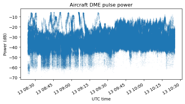
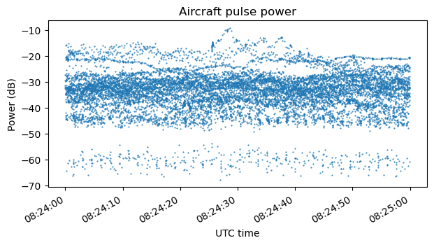
The following plots show the amplitudes of the pulse pairs detected in the air-to-ground channel, in linear and dB units. There is a wide dynamic range, from signals reaching -6 dB when an aircraft flies close to the receiver to signals around -60 dB, which probably correspond to aircraft which are very far away.

For convenience, here are the ground station and aircraft amplitude measurements again. It is apparent that small pulses in the ground-to-air frequency only appear when there are aircraft signals above a certain amplitude (for instance, there are no small pulses around 9:15 UTC), and the amplitude of these small pulses is somewhat proportional to the aircraft pulse amplitudes. However, besides this correlation, I don’t have more clues about the nature of these weak pulses, given that they don’t appear at the same time than aircraft pulses in the air-to-ground channel.
Here is a detail of the aircraft pulse power during one minute near the beginning of the recording. In this part of the recording is where the weakest aircraft pulses, at around -60 dB, are detected.
This is one of the pulse pairs below -60 dB of power. This shows that gr-dme has correctly detected this pulse rather than having mistaken some interference for a weak pulse.
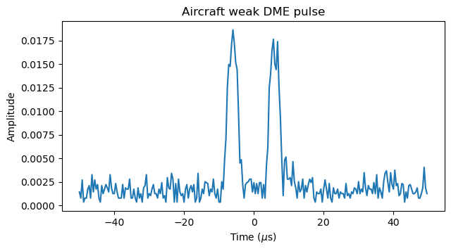
I haven’t done any tests injecting weak artificial DME pulse pairs into gr-dme to find its detection threshold. Given that aircraft that are too far away from this VOR-DME station will not use it, probably there are no DME signals in the recording that are weaker than these -60 dB signals. In particular, any aircraft using the VOR-DME station will be in line-of-sight in the receiver, since the VOR-DME station and receiver were only a few km away.
Transponder replies delays
Now we turn to the main goal of this post, which is to calculate the time difference between the reception of an aircraft pulse pair and the reception of the corresponding pulse pair transmitted by the ground station. In the previous post I already mentioned the geometric considerations for this. A DME transponder introduces a delay of 50 μs in the retransmitted pulse pair. The baseline joining the DME ground station and my receiver corresponds to a light-time delay of approximately 15 μs. Therefore, the range of delays that we expect to measure are between 50 μs and 80 μs (50 μs plus twice the baseline length). The delay can be understood as a time difference of arrival (TDOA) measurement between the DME ground station and my receiver plus a constant offset equal to 50 μs plus the baseline length.
In order to compute these delays, the first thing I do is to identify, for each aircraft pulse pair, which are the ground stations pulse pairs that appear at delays between 45 and 85 μs (I’m giving a 5 μs margin on the range of delays we expect a-priori from the geometry). A naïve implementation of this search is \(O(nm)\), where \(n\) is the number of aircraft pulses and \(m\) is the number of ground station pulses. However, since we have the lists of timestamps for the aircraft and ground station pulses ordered in time, we can write a search that is \(O(n + m)\). This efficient search algorithm is still quite slow in native Python (\(n + m\) is around 7 million here), but Numba compiles it to a very fast function.
In principle, for each aircraft pulse pair we expect to find a corresponding ground pulse pair within this 45 to 85 μs delay window. However, there might be multiple such pulse pairs or none. In fact, for 13% of the aircraft pulses there is no matching ground station pulse. I imagine that part of these happen when the transponder is sending the Morse identification, because then it ignores aircraft interrogations. I haven’t studied if the ignored pulses outside of the Morse identification intervals are always weak (so my receiver could be sensitive enough to detect them but the ground station not) or if there is another reason why the ground station might be ignoring these pulses. For 87% of the aircraft pulses we find a single matching ground station pulse within the expected delay window. There are only three aircraft pulses for which two ground station pulses are found in the expected window, and none for which three or more pulses are found. Perhaps the second pulse in these three cases is a squitter pulse that randomly just happened to appear very close to the transponded pulse. In any case, we can safely ignore these, since they are very few data points.
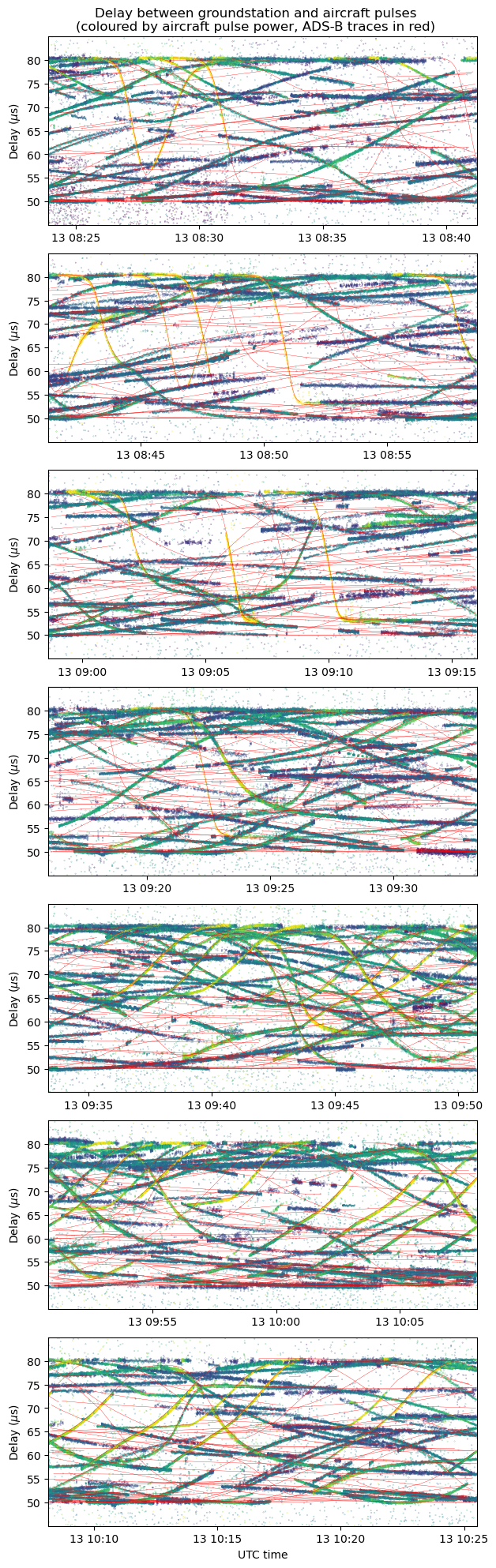
Now we represent these delays in a plot. For each aircraft pulse we plot a point in a time-delay plot using as time the reception time of the aircraft pulse and as delay the delay of the corresponding ground station pulse (for the three cases in which there were two ground station pulse candidates, the first candidate is taken, and for aircraft pulses without a corresponding ground station candidate nothing is plotted). The colour of the point represents the aircraft pulse power in a dB scale using the Viridis colormap and a colormap range between -50 and -15 dB.
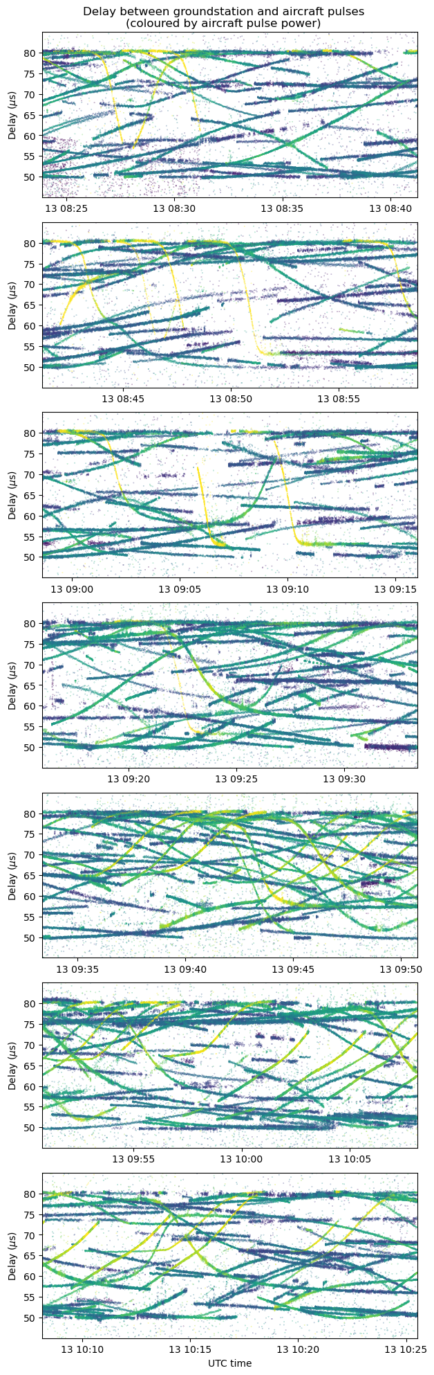
When I first saw these plots I was quite surprised. There are some many aircraft! These can be identified by their different delays. Each aircraft traces a different line in the plots as it moves and its TDOA changes. Specially at rather busy moments around 9:45 UTC I can count around 25 aircraft using this VOR-DME station simultaneously. In the previous plot I was commenting that the CNR VOR-DME that I’m using is now part of only very few instrument procedures. With time all these procedures are slowly shifting from using VOR-DME to RNAV (GNSS navigation). I expected that a few aircraft taking off from the Madrid Barajas airport might still be tuning to this VOR-DME. However, as we will see below in more detail, aircraft flying around this area often tune one of their two VOR-DME receivers to this station, even if it is not a part of their instrument procedure or airway, just to get a cross-check on their location.
The second thing that stands out is that there is a “background” of points that don’t correspond to any of the aircraft traces. I think that these are caused by aircraft pulses that the transponder ignores but for which there is a squitter pulse in the window we are searching just by chance. With a squitter rate of 700 pulse pairs per second and a 40 μs search window, the probability of finding a squitter pulse pair in the window is 2.8%. I haven’t tried to estimate if the number of “background” points that we’re seeing roughly matches this estimate.
When interpreting these delay plots, it is good to have some geometric intuition. For an aircraft far away from the baseline the delay (or TDOA) measurement indicates the angle that the aircraft makes with the baseline (more precisely the cosine of the angle). In this case the baseline is rather short (4.58 km), so most aircraft are far enough away for this to be true. The baseline is roughly oriented in a north-west to south-east direction, with the DME ground station north-west of the receiver. Thus, aircraft which are north-west of the baseline will have a delay around the minimum of 50 μs, aircraft which are south-east of the baseline will have a delay around the maximum of 80 μs, and aircraft which are either north-east or south-west of the baseline will have a delay around 65 μs.
Obtaining ADS-B data
The next step in the analysis is to compare this plot of delays with the delays calculated from the positions of the aircraft in ADS-B data and the known locations of the DME ground station and receiver. In a post I wrote back in 2018 I used the historical data at adsbexchange.com. Apparently, back then you could download their historical data for free for personal use (they recommended a very small donation to the project to cover bandwidth costs). Now you need to go through a “contact us” form if you want to download historical data. It seems their focus has shifted strongly to selling data and API access.
When researching what other sources of ADS-B data I could use for this post, I have felt that the scene of internet ADS-B data providers has become much more commercial than some years back. Luckily, I found that adsb.lol provides historical ADS-B data as per-day artifacts you can download from Github for free. This is just the kind of thing I wanted. As we will see, their data is not great, but it is still quite useful, so I’m glad this project exists. However, it seems that in 2024 we’re in a situation in which for this experiment I would had been better off using my own ADS-B receiver to collect data while doing the recording than trying to get it later from the internet. This makes me a little sad.
With the adsb.lol historical data we get “traces” JSON files for each ICAO hex ID with the data for a full day. This is quite a lot of data, even with the JSON files compressed with gzip (1.7 GB for 2024-07-13). The first step is to down select this data to only aircraft we might be interested in. For this I have written a simple “geofencing” script that copies to another folder the traces files that happened to have position data within a certain latitude and longitude box in a certain time window. I’ve used the box between 39ºN and 42ºN latitude and 5.5ºW and 1ºW, which corresponds to a good chunk of central Spain, and the time window corresponding to the recording. This gives us only 357 aircraft, with 25 MB of gzip-compressed data.
Comparison of DME delays and ADS-B data
With the ADS-B data we can compute the expected delay for each aircraft. We could do a number of things with this. We could plot the delay traces calculated with ADS-B data on top of the plot of DME pulse delays shown above to check that everything is correct. We could identify individual traces of DME pulse delays and find their corresponding aircraft and trajectory.
To plot the ADS-B delay traces on top of the DME pulse delays, we need to decide which set of aircraft to plot. I tried to come up of different heuristics for which aircraft might be using the CNR VOR-DME, but none of them worked very well. In the end I have decided to plot all the aircraft that are above 1º elevation at the receiver location. This gives a somewhat busy plot, and certainly many of the aircraft that are plotted are not using this DME. However, setting a higher elevation mask or using other heuristics tends to miss aircraft that do appear in the DME data.
The resulting plot is shown here. Each trace of ADS-B data is shown in red. The ADS-B traces are shown as lines by joining the points in the JSON data, but if there is a gap of more than 100 seconds without data, the line is broken. We can already see in this plot that many ADS-B traces suddenly stop for some reason. This will be clearer when we look at individual aircraft.
Most of the traces formed by DME pulses have a corresponding ADS-B trace that they follow quite closely. However, there are a few aircraft that have DME traces but do not have any counterpart in the ADS-B data. I think that adsblol.com is missing the data for these, as I don’t think that these aircraft wouldn’t be transmitting ADS-B. I’m not sure if the problem with adsblol.com is lack of receiver coverage. All the aircraft we see in the DME plot are aircraft that I could receive with my set up and that the CNR VOR-DME could also receive, so any reasonable ADS-B receiver in the Madrid metropolitan area would have been able to receive them as well.
Study of individual aircraft
A look at the traces in the DME delay plots shows that traces with the same shape appear at different times. These correspond to different aircraft flying along the same route. Their TDOA versus time looks the same, just offset in time. In this section I will pick a few exemplary traces and show the route of the corresponding aircraft. In principle one could devise an algorithm to automatically identify the aircraft corresponding to some particular DME trace, but I’ve been finding these manually (specially by looking at aircraft which were at a high elevation in the moment when the aircraft DME signal was strongest).
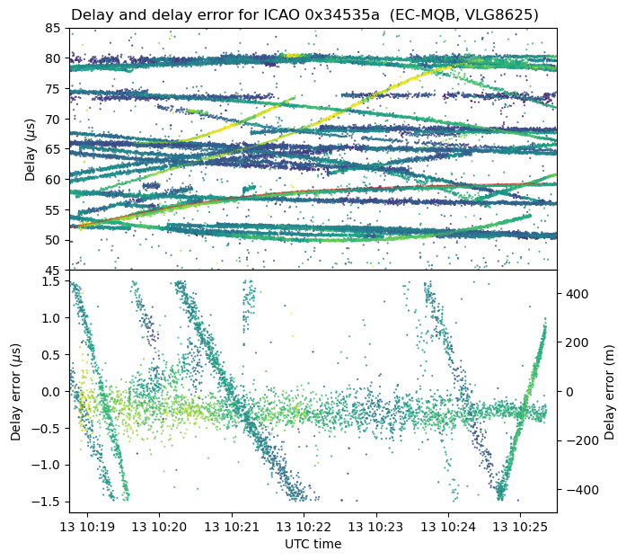
The first aircraft is the one making a parabola shape near the beginning of the recording. There is at least another example of this trace in the recording. The figure below shows on the first panel the DME pulse delays for the time range of interest, and the ADS-B trace for this aircraft. On the second panel, the ADS-B trace is subtracted from the DME traces to yield a measurement of the delay error.
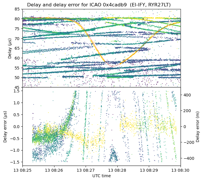
As we will also see with the other examples, there seems to be a constant error of around 0.25 μs in the delay. This is perfectly within the tolerance of a DME transponder. The FAA specifications say that the transponder should not contribute more than 0.5 μs to the total error budget. The axis on the right of the delay error plot shows the corresponding values in metres. This scale corresponds to multiplying by the speed of light. When the transponder is used in the normal way by an aircraft to determine the range, the scale needs to be divided by two, because the aircraft is measuring the round-trip time to determine the one-way range.
It is also apparent that there is also a delay error that is proportional to the derivative of the delay versus time curve. This suggests a small error in the timestamps of the data. I don’t remember if I synchronized my laptop using NTP before recording (I synchronized it at home, surely), but I also don’t trust the timestamps in this ADS-B data so much.
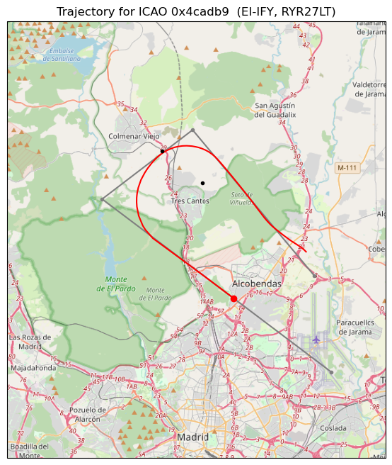
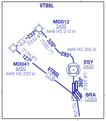
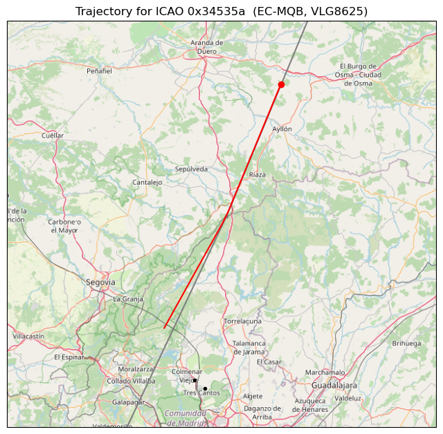
The trajectory for this aircraft is shown here. The aircraft is taking off from Madrid Barajas runway 36L and flying the VTB6L SID (instrument departure procedure). This SID is flown by southbound aircraft and takes them in a U-turn over the CNR VOR-DME as they ascend, to overfly the BRA VOR-DME at Barajas airport and then head south to the VTB VOR-DME. In particular, this aircraft is flight RYR27LT, a Ryanair flight from Madrid to Tenerife. The waypoints for this route are shown in grey, while the aircraft trajectory according to ADS-B is shown in red. The final position of the aircraft is shown in red. At this point, the ADS-B data is lost, and there is no reason why it should be. Looking at the DME plots, the aircraft continues to use the CNR VOR-DME for a little while longer, but its trace becomes intermixed with those of other aircraft.
Now that we know the route of the aircraft, it is clear why its DME trace looks like a parabola. Interestingly, the DME signal stops while the aircraft is overflying the CNR VOR-DME. I don’t know why this happens. Certainly the DME ground station antenna doesn’t have much gain in the vertical direction, but the aircraft isn’t too high, so the ground station should still be able to receive its signal.
The next example DME trace sweeps from 80 μs to 50 μs with a sigmoid curve that has some peculiar shape in the bottom half. It is also relatively long, with the aircraft signal fading away at the end. This kind of trace appears at least two times in the DME data. It also appears another time in the ADS-B data without a corresponding DME trace. This means that the aircraft wasn’t tuned to the CNR VOR-DME.
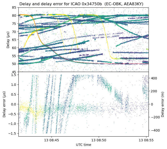
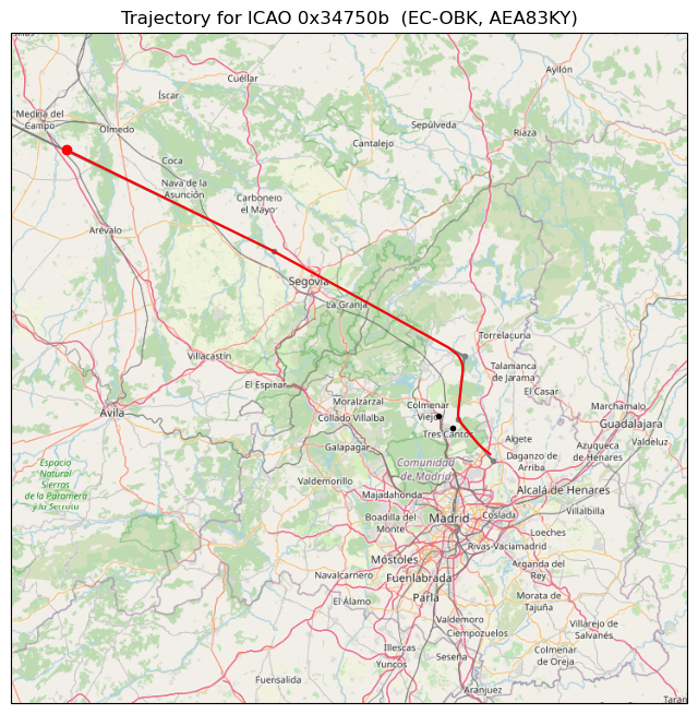
The figure below shows the trajectory flown by this aircraft. We can still receive its DME signal at a distance of approximately 120 km. The aircraft is departing from Madrid Barajas runway 36L using the ZMR7L SID. This is flown by aircraft departing north-west. It involves first turning left to take the aircraft out of the way of the traffic departing runway 36R (there is an alternative ZMR3X departure which first turns slightly right, so it potentially conflicts with traffic from runway 36R), then flying roughly due north, and finally flying northwest to the ZMR VOR-DME. This particular aircraft is flight AEA83KY, an Air Europa flight from Madrid to A Coruña.
Another example is a DME trace that goes from 80 μs to 55 μs in a sigmoid curve quite fast (the transition happens in slightly more than one minute). There are several cases like this in the DME data. The strong aircraft pulses indicate that the aircraft is near the receiver in this part of its route.
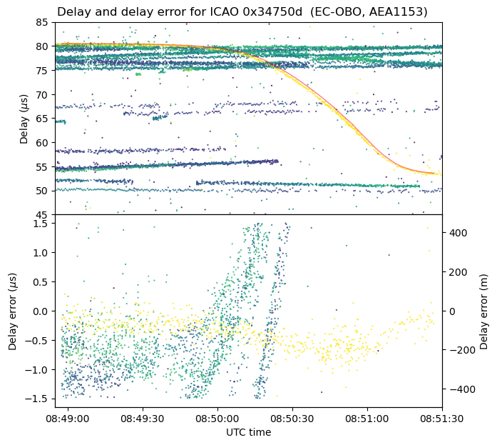
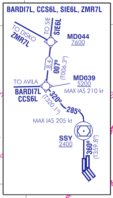
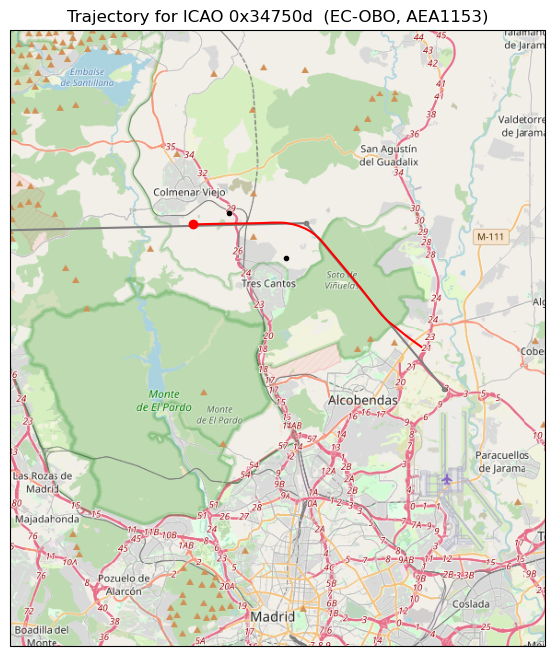
The route for this aircraft is shown below. It is flying the BARDI7L or CCS6L SID (see the SID chart inset shown above). This route is used by aircraft departing from Madrid Barajas runway 36L and flying due west (to the BARDI nav point) or south-west (to the CCS VOR-DME). The SID begins in the same way as ZMR7L, but the aircraft turns west instead of north and then north-west. This particular aircraft is flight AEA1153, an Air Europa flight from Madrid to Lisbon.
Aircraft on this route fly over the baseline, close to the CNR VOR-DME. Looking at the different examples of aircraft flying this SID in the DME delay plot, it is apparent that some aircraft stop tuning to the CNR VOR-DME as soon as they pass over it, while others continue tuning to it for some more minutes.
An interesting example is the following DME trace that changes from around 57 μs to 75 μs in a sigmoid curve.
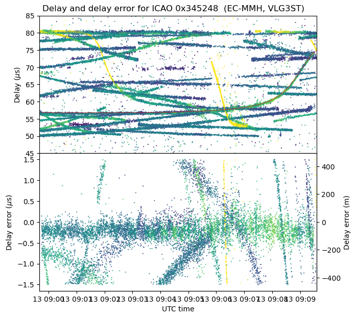
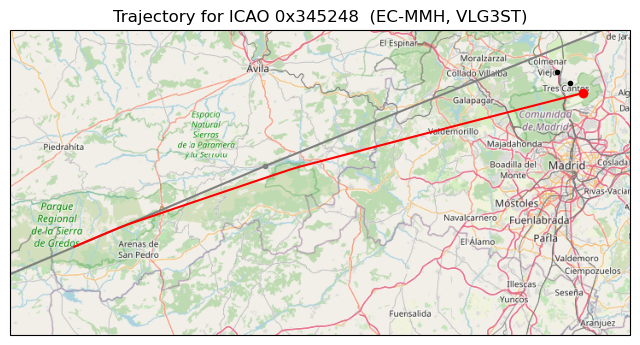
This trace corresponds to flight VLG3ST, a Vueling flight from Lisbon to Barcelona. Usually it seems to fly along airway N870, which would take it slightly north of the CNR VOR-DME, as depicted by the grey line that shows the route waypoints. However, this particular day the flight took a shortcut for some reason and flew slightly south of this airway. Note that these two trajectories would cause completely different DME delay traces, because one goes through the north-west extension of the baseline and another through the south-east extension of the baseline.
The following DME trace begins slightly above 75 μs, then goes slightly up and finally goes down to 55 μs in a sigmoid curve. There are a few examples like this in the recording.
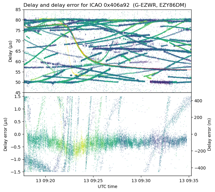
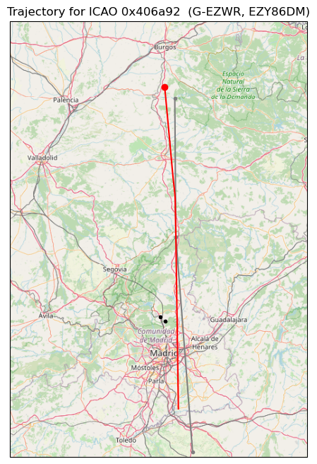
This trace corresponds to an aircraft flying on a south to north trajectory, which explains the slight increase in delay at the beginning. It is travelling close to airway N865, which is shown as a grey line, but not quite exactly on the airway. In this case, the flight is EZY86DM, an Easy Jet flight from Malaga to Bristol.
An important example is the following DME trace, which increases from around 57 μs to 72 μs in an almost straight line. This kind of trace appears many times after 9:40 UTC, and is responsible for part of the high traffic observed around 9:45 UTC.
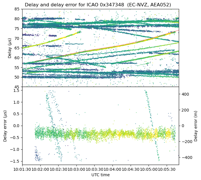
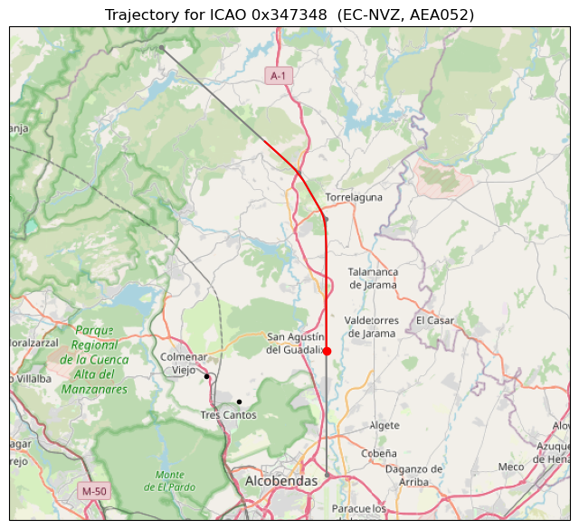
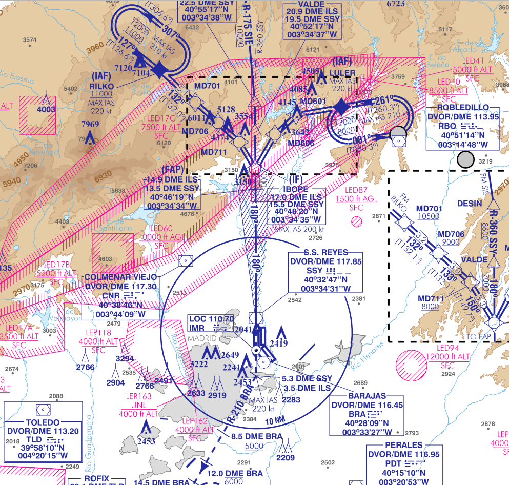
The trajectory of this aircraft is shown below. It is flying an ILS approach to runway 18R. In this case the flight is AEA052, an Air Europa flight from Havana to Madrid. Something interesting has happened around 9:30 UTC. Barajas normally operates in a northbound configuration, with aircraft taking off runways 36L and 36R, which are parallel runways in the north half of the field, and landing in runways 32L and 32R, which are parallel runways in the south half of the field. We have already seen examples of aircraft taking off runway 36L. However, depending on wind conditions Barajas can change to a southbound configuration, in which runways 18L and 18R (36R and 36L in the opposite direction) are used for landing and runways 14L and 14R are used for take off. This configuration change is what has happened here. It seems that many aircraft flying the ILS approach to runway 18R are using the CNR VOR-DME, which explains the increase in traffic seen in the delay plots.
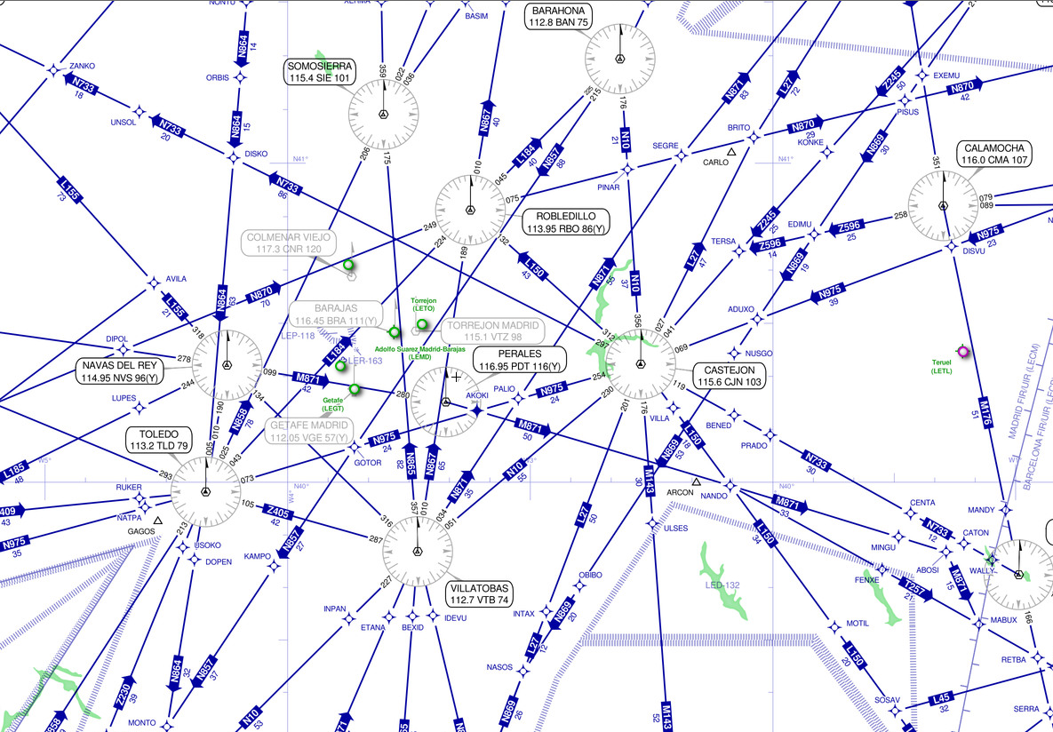
The following figure shows the ILS Z approach procedure to runway 18R. The CNR VOR-DME is not part of the procedure (the DME measurements which are referenced in the approach plate are from the SSY and BRA VOR-DMEs and from the ILS), but pilots might still decide to tune to it as a convenient reference when flying the approach.
The last example shows a trace that increases from around 52 μs to 57 μs. There are a few other examples of traces that only cover a small delay range like this.
The flight number for this aircraft has been misidentified by my code (which selects a flight number that appears anywhere within the window where the recording was made). The flight is actually VLG8624, a Vueling flight from Tangier to Paris. It seems to be flying along airway N858, which is shown as a grey line.
Conclusions
In this post I have presented a GNU Radio DME receiver that detects and measures DME pulse pairs. Using the output of this receiver, we can match aircraft pulse pairs with their corresponding ground transponder replies, and measure the time difference of their arrival at the receiver. This delay measurement is equivalent to a TDOA measurement of the aircraft with respect to the baseline formed by the receiver and the DME ground station. In a plot of the delay versus time of the DME pulse pairs, different aircraft and their trajectories can be identified by the shapes of the traces that they form. I have shown how these traces can be matched manually to aircraft position data from ADS-B.
There is much more that could be done with this data. The idea of separating automatically the different traces in the delay plot is quite appealing, but it seems a tricky problem. Perhaps there are suitable machine learning algorithms that can classify the points shown in these plots according to the curves that they form. This kind of algorithms would enable other applications, such as automatically matching aircraft traces to ADS-B data, detecting anomalies, such as aircraft which are not present in ADS-B, and classifying aircraft pulses to study each aircraft separately.
It is also possible to do a deeper study of the DME signals. For instance, the precise pulse shape can be measured by aligning and averaging multiple pulses, as it is often done with pulsars in radio astronomy. The average pulse rate over time can be studied. For the aircraft we should be able to distinguish between search and tracking modes, while for the ground station we should be able to classify the pulses into interrogation responses and squitter, and measure that these follow the expected rates. For aircraft pulses it is also possible to study whether they follow a certain regular period, and if the pulse shape and period can serve to identify a certain aircraft DME model. A regular pulse period would perhaps also give a way to separate the pulses from different aircraft.
Code and data
The IQ recording of DME signals used in this post can be found in the dataset “Recording of Colmenar (CNR) VOR-DME air-to-ground and ground-to-air DME channels” in Zenodo. The GNU Radio receiver is in the gr-dme out-of-tree module. The design of the DME pulse shape matched filter has been done in this Jupyter notebook. The main study is carried out in this Jupyter notebook. The data files, produced by gr-dme, as well as the aircraft ADS-B traces selected with the geofencing algorithm are also found in the repository.
This is fantastic Daniel. Thank you for sharing!