On Sunday March 2, Firefly Aerospace’s Blue Ghost Mission 1 successfully landed on Mare Crisium, becoming the first NASA CLPS mission to perform a fully successful lunar landing. Congratulations to all the team at Firefly for this huge achievement.
Both AMSAT-DL and CAMRAS covered this event live, by receiving the S-band beacon from the lander with the 20 m antenna in Bochum Observatory and the 25 m Dwingeloo radiotelescope respectively, and streaming the waterfall of the signal in YouTube.
In this post I do a quick analysis of the Doppler of the signal received at Bochum and Dwingeloo. Part of the goal of this is to try to answer a question of Jonathan McDowell, who asked if it was possible to determine the exact second of the touchdown from this data. The answer is that this is probably not possible, since for a soft touchdown there is no significant acceleration at touchdown that can be identified in the Doppler curve.
The raw IQ data recorded by AMSAT-DL is not publicly available. The data recorded by CAMRAS can be found here.
The S-band telemetry downlink of BGM-1 has a carrier frequency of approximately 2251.113 MHz. Most likely it is GMSK at 15625 baud. There are a number of very similar waveforms which are related to MSK and OQPSK modulations, and without detailed analysis it is difficult to tell them apart (see for instance my comments about the Orion OQPSK telemetry). In any case, for the purposes of this post, we can treat the waveform as GMSK.
Since GMSK is a suppressed carrier modulation, some signal processing is required to extract and measure the carrier frequency. There is a trick to do this, which consists in squaring the signal (i.e., computing \(x(t)^2\), where \(x(t)\) is the time-domain signal). This will cause spectral lines to appear at \(2 f_c \pm f_s/2\), where \(f_c\) denotes the carrier frequency and \(f_s\) denotes the symbol rate.
To realize why this happens, it is easier to think first about an MSK waveform. Assuming that the carrier frequency is zero, for an MSK waveform the phase of the signal moves \(\pm\pi/2\) radians at constant speed during each symbol period. Therefore, at each symbol boundary the signal is always at one of four points on the unit circle spaced by \(\pi/2\) radians. When we square the signal, we obtain something that moves \(\pm \pi\) radians at constant speed during each symbol period. Therefore, the squared signal is always at one of two opposite points on the unit circle at each symbol boundary. The symbols in which the squared signal moves by \(\pi\) radians correspond to a half-period of a CW carrier of frequency \(f_s/2\). Moreover, all these CW carriers have the same phase. Therefore, they all contribute to the presence of a spectral line at frequency \(f_s/2\). Likewise, the symbols in which the squared signal moves by \(-\pi\) radians contribute to a spectral line at frequency \(-f_s/2\).
An important remark is that the MSK signal (without squaring) does not have any spectral lines (when the data is random), because even if each symbol corresponds to a quarter-period of a CW carrier of frequency \(\pm f_s/4\), half of these CW carriers have the opposite phase compared to the other half, so they cancel each other out, and in average there is no net contribution to spectral lines at \(\pm f_s/4\).
Having understood what happens by squaring an MSK signal at a carrier frequency of zero, it is easy to figure out all the rest. If the MSK signal is at carrier frequency \(f_c\) instead, then the tones at \(\pm f_s/2\) are offset by \(2f_c\), because we are squaring everything, so the carrier frequency gets multiplied by two. If the signal is GMSK rather than MSK, then almost the same reasoning applies. The only difference is that the speed at which the phase of the signal covers a distance of \(\pm \pi/2\) during a symbol period is not constant. The average speed is the same, though, so there is still a positive contribution to spectral lines at \(\pm f_s/2\) in the squared signal.
Note that this trick does not work for all the waveforms in the MSK/OQPSK family. For instance, for OQPSK with a rectangular pulse shape, the signal squared is BPSK at twice the symbol rate, so there are no spectral lines.
The squaring trick has also been used by Cees Bassa, from the CAMRAS team, to extract not only the carrier frequency of the signal, but also to visualize the reflections of the signal on the lunar surface. These reflections have a different Doppler compared to the direct signal, but since the GMSK signal is broadband, they are usually invisible unless some signal processing is done to reveal these spectral lines.
To measure the carrier frequency of the GMSK signal, I use the following GNU Radio flowgraph. This particular flowgraph is for processing the Bochum recording, which has a sample rate of 1041666 sps. The Dwingeloo recording has a sample rate of 4 Msps and is processed with a slightly different flowgraph.
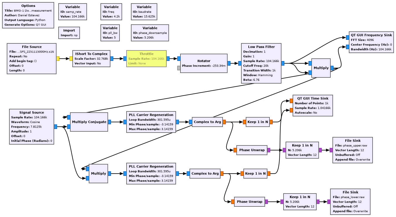
First the signal is downconverted to baseband and low passed filtered. The squaring trick causes squaring losses, so it is good to remove unneeded noise bandwidth before squaring. After squaring the signal, CW tones of \(\pm f_s/2\) are used to downconvert the two spectral lines to baseband, and a PLL is locked to each of them. The unwrapped phase of each PLL is recorded to a file, using the Phase Unwrap block from gr-satellites. This block outputs unwrapped phase as an int64_t that counts integer cycles and a float that counts the fractional part of the cycle in units of radians.
Only one phase measurement for every 5206 samples is recorded. This gives a phase measurement rate of almost 20 Hz, which is more than enough for later analysis. The PLL bandwidth is set to 5 Hz. The PLL blocks in GNU Radio are based on the control_loop class, which sets its loop coefficients using some formulas derived from a continuous time analysis. I have never tested how accurately the desired noise bandwidth is actually achieved (see my post about PLL loop coefficients for another approach at control loops that uses discrete time analysis to achieve the noise bandwidth accurately).
The output from this GNU Radio flowgraph is analyzed in a Jupyter notebook. The unwrapped phase measurements are further decimated by a factor of 4 to obtain a measurement rate of almost 5 Hz. Frequency is computed by differentiating the phase in these 0.2 second intervals. This gives smoother plots than the 0.05 second intervals corresponding to the 20 Hz rate, while still having enough time resolution to capture brief events. The carrier frequency is estimated by computing the average of the frequencies of the two spectral lines, and by dividing by 2 (this division is needed because the signal squaring multiplies the carrier frequency by 2).
The following plot shows the carrier frequency of the telemetry signal as observed by the Bochum and Dwingeloo groundstations. Note that the two recordings have a rather different time range. The Bochum recording contains a large period of an orbit (which has a Doppler curve which is approximately sinusoidal), and shows the beginning of the power descent at 08:22:26 UTC (this can be identified by the kink that the start of the thrusters acceleration produces on the Doppler curve). The Dwingeloo recording begins during the power descent. Both recordings cover the landing, at around 08:34 UTC, and have a few minutes of data of the spacecraft stationary on the lunar surface.
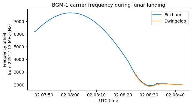
The frequency in this plot is depicted as an offset from 2251.113 MHz. As we will see below, this is approximately the carrier frequency of the signal once the spacecraft is landed, if we factor in the Doppler due to the relative motion of the Moon and the groundstations.
The next figure shows a zoom to a few minutes around the landing, which happened approximately at 08:34 UTC. As expected, the data from both groundstations looks very similar, but there is an offset of approximately 60 Hz between them. I will speak more about this later.
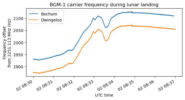
The lander has already been spotted by the LRO NAC, and its coordinates are given as 18.562ºN 61.810ºE -3650 m elevation. The elevation of Earth at this location was 26.3 deg. Using this, we can compute that, for a motion that is purely vertical, a Doppler shift of 1 Hz corresponds to a velocity of 0.3 m/s. A negative Doppler shift corresponds to a downwards vertical velocity.
The Doppler shift, however, measures velocity along the line-of-sight vector, and there is no way to distinguish vertical and horizontal movement from the Doppler curve alone. Nevertheless, it is good to keep this conversion factor between Doppler and velocity in mind. Using it, we see that the 150 Hz change that is present in the plot above corresponds to a vertical velocity of approximately 45 m/s.
If we zoom in more to the region around the touchdown, we see that the frequency is almost constant after 08:34:30 UTC, except for a sudden downwards jump that happens some seconds before 08:35 UTC. I don’t think this jump corresponds to physical movement, because geometrically it does not make sense. It would imply that just before touchdown the vertical velocity is slightly positive, and then it suddenly becomes zero (assuming that the spacecraft is landed at and after 08:35 UTC). The sudden jump is more likely to be caused by some effect of the electronics of the spacecraft oscillator.
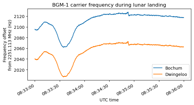
Assuming that the frequency at around 08:34:30 UTC corresponds to the spacecraft stationary at the surface, we see that the Doppler was -60 Hz slightly after 08:33:30 UTC. This would correspond to a downwards velocity of 18 m/s if only vertical movement was involved. The Doppler slowly becomes more positive, until smoothly becoming almost constant. This supports a rather smooth deceleration and soft landing, which makes it quite difficult to identify the touchdown as a distinct event in the Doppler curve, specially because the transmitter frequency is not very stable.
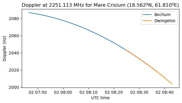
We can perform a more accurate analysis by computing the Doppler caused by the relative motion between the landing site and the groundstations and subtracting it from the observed data. I have used GMAT to compute the relative positions and velocities of the groundstations. The plot of this “lunar Doppler” can be seen below. It is mainly caused by the Earth rotation, and follows the downwards arc of a sinusoid because the Moon is rising from the point of view of the groundstations. The two Doppler curves are very similar because the groundstations are just 160 km apart.
The plot of the carrier frequency around the landing moment with the contribution of lunar Doppler removed is shown here. We can see that some of the downwards slope of the frequency of the transmitter once it is stationary was caused by the lunar Doppler, but there is still a noticeable downwards slope present. This is most likely caused by a change in the temperature of the spacecraft oscillator, and shows that the transmitter frequency is not too stable.

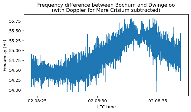
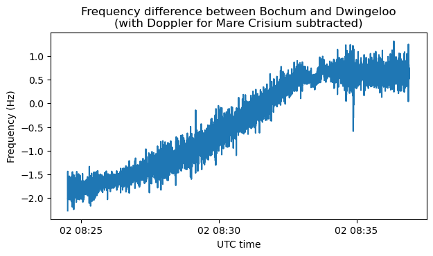
Now that we have subtracted the contribution of the lunar Doppler, the observed frequency in both groundstation should be identical, specially because the groundstations are close (with distant groundstations there might be a small difference due to parallax). However, there is a difference that varies between 54.5 Hz and 55.5 Hz, as shown by the following plot. I don’t know the details of all the clocking in the two groundstations, but this difference, and specially the fact that it varies over time, suggests that there is something that is not properly locked to GPS time in at least one of the groundstations.
High-quality footage of the landing has recently been released by Firefly. Since many lunar surface features are visible in the video, it might be possible to estimate the lander’s velocity with respect to ground. The Earth is also visible in several of the takes. It would be interesting to compare this video with the Doppler data.
All the materials used in this post can be found in this repository.
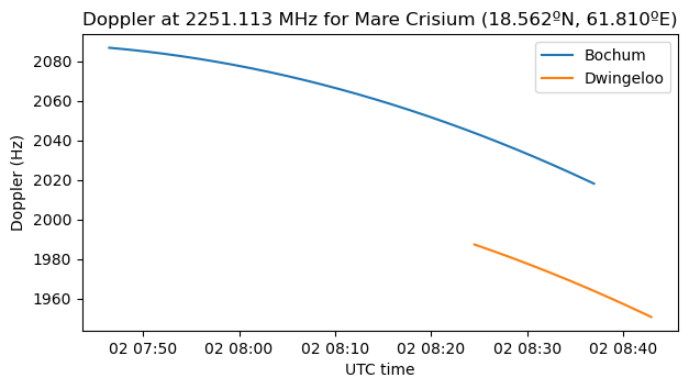
Update 2025-04-25: Leif has noticed an error in this post. The expected lunar Doppler observed at Dwingeloo was wrong due to a copy & paste error that I made in the code. I have updated the Jupyter notebook to correct this mistake.
After correcting this error, it turns out that there is a significant difference between the predicted lunar Doppler for Bochum and Dwingeloo. In the post above I basically got the same curve and explained this as both stations being just 160 km apart. However, Earth rotation Doppler is a sinusoidal curve whose amplitude is proportional to the cosine of the latitude. The quotient of the cosines of the latitudes of Bochum (51.427 deg) and Dwingeloo (52.812 deg) is about 1.03. This means that the Doppler curve for Bochum would have about 3% more amplitude than the curve for Dwingeloo. From the plot we can see that the amplitude of the curve for Bochum is slightly larger than 2 kHz. Since 3% of 2 kHz is 60 Hz, the difference between the two Doppler curves in the plot below is completely expected.
With this mistake corrected, now the Doppler-corrected BGM-1 carrier frequency measured at each station almost coincides.
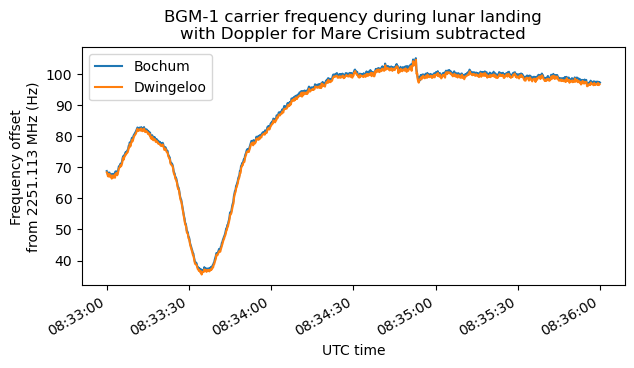
The difference between the Bochum and Dwingeloo measurements is now quite small, on the order of 1 Hz. This is about 0.7 ppb, so it is well within the frequency stability and accuracy that we would expect for the Bochum GPSDO.
This is excellent work. Thank-you!
Hello Daniel – this is very interesting thanks. I wonder if you might be miscalculating the lunar_doppler_dwingeloo_interp for the Dwingeloo site. It seems like you calculate the interpolation twice using the same value before the final close-parenthesis: lunar_doppler_bochum is used for both lunar_doppler_bochum_interp and lunar_doppler_dwingeloo_interp
See snapshot from your github page.
“`
lunar_doppler_bochum_interp = np.interp((t_freq – t_freq[0]) / np.timedelta64(1, ‘s’),
(lunar_doppler_t – t_freq[0]) / np.timedelta64(1, ‘s’),
lunar_doppler_bochum)
lunar_doppler_dwingeloo_interp = np.interp((t_freq_dwingeloo – t_freq[0]) / np.timedelta64(1, ‘s’),
(lunar_doppler_t – t_freq[0]) / np.timedelta64(1, ‘s’),
lunar_doppler_bochum)
“`
You are totally right. Thanks for noticing this error! I have added an update at the end of the post with the correction. This mistake explains the difference of ~50 Hz that I got between Dwingeloo and Bochum.