Trying to improve the performance of the demodulators in gr-satellites, I am switching to the Symbol Sync GNU Radio block, which was introduced by Andy Walls in GRCon17. This block covers the functionality of all the other clock synchronization blocks, such as Polyphase Clock Sync and Clock Recovery MM, while fixing many bugs.
One of the new features of the Symbol Sync block is the ability to specify the gain of the timing error detector (TED) used in the clock recovery feedback loop. All the other blocks assumed unity gain, which simply causes the loop filter taps to be wrong. However, the TED gain needs to be calculated beforehand either by analysis or simulation, as it depends on the choice of TED, samples per symbol, pulse shaping, SNR and other.
While Andy shows how to use the Symbol Sync block as a direct replacement for the Polyphase Clock Sync block in his slides, he leaves the TED gain as one, since that is what the Polyphase Clock Sync block uses. In replacing the Polyphase Clock Sync block by Symbol Sync in gr-satellites, I wanted to use the correct TED gain, but I didn’t found anyone having computed it before. This post shows my approach at simulating the TED gain for polyphase matched filter with maximum likelyhood detector.
Andy gave an Octave simulation for the Müller and Muller, and Gardner TEDs that accompanies an example flowgraph for Symbol Sync. After reading the code involved in a polyphase matched filter with the Symbol Sync block, I decided to follow a different approach. The construction of the polyphase filter is a bit involved, especially the normalization of the derivative filter taps, which I find a bit odd. To avoid making mistakes and getting an implementation which doesn’t match GNU Radio, I decided to use GNU Radio for the simulation instead of implementing a standalone simulation.
To perform the simulation I need to use some GNU Radio classes that aren’t available on the API, so the source code of GNU Radio is needed to build the simulation, which is written in C++.
To explain my simulation, I first need to explain some approximations and simplifications that can be made with TED. The case I am interested in is a polyphase matched filter for a PSK signal of amplitude one. The TED I am using is the complex ted_signal_times_slope_ml, which can be described by the formula\[\frac{1}{2}\operatorname{Re} x_n\overline{x’_n},\]where \(x_n\) denotes the signal after matched filtering and \(x’_n\) denotes the derivative of the signal after matched filtering (obtained via convolution with the derivative filter).
I don’t understand the motivation for the factor 1/2 in the formula above, since the real ted_signal_times_slope_ml detector uses just \[x_n x’_n.\]Therefore, the results obtained here can be applied to the real case, but the gain should be multiplied by two.
Now, the approximation goes as follows. We are interested in the derivative of\[\varepsilon(t) = \operatorname{Re} x(t)\overline{x'(t)}\]at an instant \(t = t_0\) aligned with the symbol clock. We have\[\varepsilon'(t_0) = |x'(t_0)|^2 + \operatorname{Re} x(t_0)\overline{x^{\prime\prime}(t_0)}.\]
Now denote by \(r(s)\) the raised cosine pulse, with the normalization that \(r(0) = 1\) and \(r(n) = 0\) if and only if \(n \in \mathbb{Z}\setminus\{0\}\). Then\[x(t_0 + sT) = \sum_{k \in \mathbb{Z}} a_k r(s-k),\]where \(T\) is the symbol period and \(a_k\) are the PSK symbols, which we assume to be independent random variables such that \(\mathbb{E}[a_k] = 0\) and \(|a_k| = 1\).
Thus,\[x'(t_0) = \frac{1}{T}\sum_{k\in\mathbb{Z}}a_k r'(-k).\]Since \(r'(0) = 0\), we see that the reason why \(x'(t_0)\) is non-zero in general is because of inter-symbol interference from symbols \(a_k\) with \(k \neq 0\). We decide to disregard this kind of inter-symbol interference and drop out the term \(|x'(t_0)|^2\) from the expression for \(\varepsilon'(t_0)\). This is our approximation. If following a more precise approach, we would compute\[\mathbb{E}[|x'(t_0)|]|^2 = \frac{1}{T^2}\sum_{k\in\mathbb{Z}} r'(-k)^2,\]using the fact that the variance of \(a_k\) is one.
After the approximation, we are left with\[\operatorname{Re} x(t_0)\overline{x^{\prime\prime}(t_0)} = \frac{1}{T^2}\operatorname{Re} \sum_{k\in\mathbb{Z}} a_0 \overline{a_k} r^{\prime\prime}(-k).\]Taking the expectation,\[\mathbb{E}[\operatorname{Re} x(t_0)\overline{x^{\prime\prime}(t_0)}] = \frac{1}{T^2}r^{\prime\prime}(0),\]since \(a_k\) are independent. This is the same that we would obtain if we compute \(\varepsilon'(t_0)\) for \(a_0 = 1\) and \(a_k = 0\), \(k \neq 0\), so that our signal \(x(t)\) is a raised cosine pulse adequately scaled to the symbol period \(T\).
This motivates our simulation, which is based in running a raised cosine pulse through the TED. Disregarding the \(|x'(t_0)|^2\) term produced by inter-symbol interference, this should give the same results as passing a raised cosine filtered PSK signal with random data and averaging over all the symbols.
Since we are using a polyphase matched filter, we first generate a root raised cosine pulse signal, then apply the polyphase filter to generate the match-filtered signal and derivative, and then use the maximum likelyhood detector to compute the clock phase error.
In order to compute the detector S-curve, we generate the input root raised cosine pulse at different clock phases by following a polyphase approach. A root raised cosine pulse at 100 * sps samples per symbol is generated and then decimated to sps by taking one out of every 100 samples at each offset. Here sps stands for the simulation samples per symbol.
The C++ simulation can be seen here. It uses the timing_error_detector detector and interpolating_resampler_ccf classes, which are used behind the scenes by the symbol_sync_cc class. These classes are not exported on the API, so the GNU Radio sources are required to build the simulation against the sources of these classes.
The simulation computes the TED gain at a clock phase of zero by approximating the derivative of the TED error by subtracting the errors at two close clock phases.
The following Jupyter notebook shows the output of the simulation, including the output of the matched filter, derivative filter and TED error. As a result, we get the figure below, which shows that the TED gain in units of 1/sample follows closely the curve 0.5/sps.
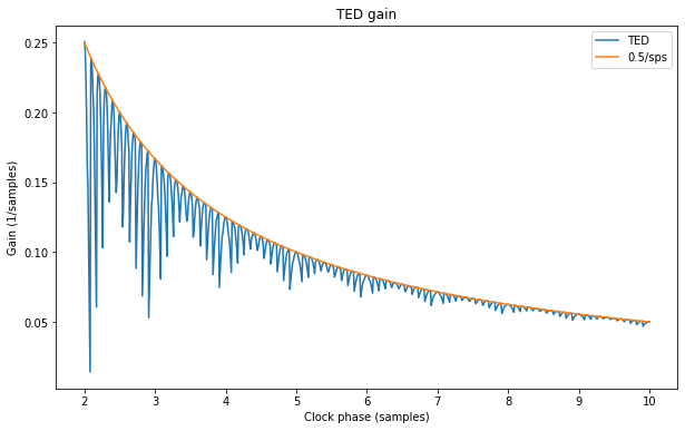
In fact, the TED gain equals 0.5/sps when the samples per symbol is of the form \(k/2\), for \(k \in \mathbb{Z}\), but is different when the samples per symbol is of the form \((2k+1)/4\), for \(k \in \mathbb{Z}\).
The conclusion is that, except when sps is small, the function 0.5/sps is a good approximation for the TED gain. This approximation is what I’m using now in the gr-satellites next branch. Note that the factor 0.5 comes directly from the factor 1/2 in the definition of the complex maximum likelyhood detector. For the real case, 1/sps should be used instead, since the real detector doesn’t include the factor 1/2.
Update 2020-02-29: I have realised that the TED gain in the Symbol Sync block should be specified in units of 1/symbol instead of 1/sample (which is what the last slide in Andy’s presentation seems to indicate). The reason for this is that the TED error, and hence the loop filter update, is computed only once per symbol, regardless of the input samples per symbol. Therefore, 0.5 instead of 0.5/sps should be used as TED gain for the conditions described in this post.
One comment