The title of this post is quite a mouthful (I couldn’t come up with anything better), so let me start by describing the particular problem that got me thinking into this sort of things.
Some days ago, I did a Python script to plot several data regarding an observation of the DSLWP-B lunar orbiting satellite. One of the plots I included was a plot of the position of DSLWP-B in the sky with respect to the Moon. An example of this kind of plot can be seen below.
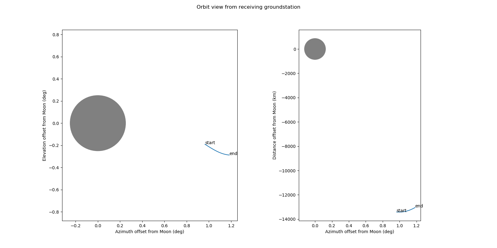
To represent the position of DSLWP-B in the sky, I chose to use azimuth and elevation coordinates, as these seemed more natural. For instance, this plot could be used for aiming an antenna, such as the 25m radiotelescope at Dwingeloo, and antennas are usually pointed in terms of azimuth and elevation.
The problem comes when trying to represent the lunar disc in these coordinates. Disregarding the flattening of the Moon (as we will do throughout this post), we can consider the Moon as a sphere of radius \(R = 1737.1\ \mathrm{km}\). Therefore, the Moon is seen on the celestial sphere as a disc of angular radius\[\alpha = \arcsin\left(\frac{R}{D}\right),\] where \(D\) is the distance from the observer to the centre of the Moon. If we set \(D\) to the mean distance between the Earth and the Moon, we get an angular radius \(\alpha\) of approximately 0.26 degrees.
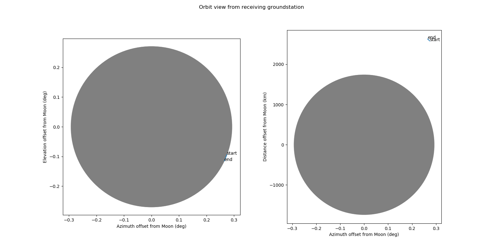
Naïvely, I drew a circle with a radius of 0.26 degrees in my plot to represent the Moon, as you can see in the figure above. I noticed this was wrong when Tammo Jan Dijkema tried to plot a grazing occultation of DSLWP-B behind the Moon’s edge. Where we expected to get the position of DSLWP-B very close to the Moon’s edge, we got the picture below.

It is not very difficult to realize what is the problem here: while a movement of 0.26 degrees in elevation does indeed subtend an angular distance of 0.26 degrees, a movement of 0.26 degrees in azimuth does not subtend an angular distance of 0.26 degrees, in general. Indeed, the angular distance subtended by such a movement in azimuth will be smaller than 0.26 degrees, and will depend on the elevation (being smaller for higher elevations). The reason for this is that the lines of constant azimuth on the celestial sphere get closer together as one approaches the zenith.
The obvious question then is: what is the shape of the Moon when plotted in these coordinates? This question can be considered more in general. Let \(S\) be a sphere in \(\mathbb{R}^3\) (where \(S\) is not necessarily centred in the origin) and write spherical coordinates\[\begin{split} x &= r\cos \theta \cos \varphi,\\ y &= r \sin \theta \cos \varphi,\\ z &= r\sin\varphi.\end{split}\] What is the set \(P\) of points in the \((\theta, \varphi)\) plane obtained by projecting \(S\) onto the unit sphere?
An equivalent question, of interest in cartography, is the following: Consider a circle on the surface of the Earth. What is its shape under an equirrectangular projection? (Note that this is only equivalent if we ignore the Earth flattening).
The answer to this question is that the shape \(P\) cannot be described in an easy way. Getting back to the setting of viewing a spherical object in azimuth and elevation coordinates, consider what happens when the object gets closer and closer to the zenith. Its projection in the azimuth-elevation plane gets deformed to compensate for the fact that the lines of constant azimuth are closer near the zenith, so the object keeps getting wider in azimuth as we move it closer to the zenith. The effect of this deformation is larger on the “top” of the object, which is nearer the zenith than the “bottom” of the object. We get an extreme case when the top of the object touches the zenith.
However, if the angular radius of the object is small and the object is not too close to the zenith (which is the case for the Moon), the shape can be approximated by an ellipse. This is simply because the spherical coordinates can be approximated by a linear map using the Jacobian, and linear maps take spheres into ellipsoids.
A way to compute this ellipse is to note that angular distances are the same as Riemannian distances on the unit sphere, and that the Riemannian metric (or first fundamental form) of the unit sphere, written in spherical coordinates, is\[ds^2 = dx^2 + dy^2 + dz^2 = (\cos\varphi)^2 d\theta^2 + d\varphi^2.\]Therefore, a disc of angular radius \(\alpha\) on the unit sphere gets mapped into an ellipse with a semi-axis of \(\alpha/\cos \varphi\) in azimuth and a semi-axis of \(\alpha\) in elevation.
There is another approach to this problem which is perhaps more elemental, since it doesn’t use differential calculus. It only uses spherical trigonometry. We want to know what is the angular distance \(\alpha\) subtended by a movement of \(\theta\) in azimuth. To this end, we consider points \(A\) and \(B\) on the unit sphere with spherical coordinates of \((0, \varphi)\) and \((\theta, \varphi)\) respectively. Without loss of generality, we consider that \(\varphi \geq 0\), so that the points lie on the northern hemisphere. We denote by point \(C\) the north pole.
Now, if we consider the spherical triangle with vertices \(A\), \(B\) and \(C\), and denote by \(a\), \(b\) and \(c\) the lengths of its sides (where \(a\) is the length of the side opposing the vertex \(A\) and so on), we have that \(a = b = \pi/2 – \varphi\) and \(c = \alpha\) is precisely the angular distance between the points \(A\) and \(B\).
Abusing notation, we denote also by \(A\), \(B\) and \(C\) the angles at each of the vertices. We have \(C = \theta\). Using the spherical law of cosines\[\cos c = \cos a \cos b + \sin a \sin b \cos C\]and the fact that \(\cos(\pi/2 – x) = \sin x\), we get\[\tag{1}\cos \alpha = \sin^2 \varphi + \cos^2\varphi \cos \theta.\]
From this we get that the semi-axis in azimuth of the ellipse representing a disc of angular radius \(\alpha\), whose centre is at a latitude of \(\varphi\), should be\[\tag{2}\theta = \arccos\left(\frac{\cos \alpha – \sin^2 \varphi}{\cos^2 \varphi}\right).\]
While this value is different from the value of \[\tag{3}\theta = \frac{\alpha}{\cos \varphi}\] that we had obtained using differential geometry, it is possible to recover (3) by using in (1) the approximation \(\cos x \approx 1 – x^2/2\) for \(\cos \alpha\) and \(\cos \theta\).
Even though (3) is a simpler expression than (2), I prefer to use (2), because it involves no approximations. Using (2), we get the vertices of the ellipse exactly at the boundary of the shape \(P\), since the vertices have an angular distance of \(\alpha\) to the centre of the ellipse. We know, however, that \(P\) is not exactly an ellipse (in other words, the angular distance of the remaining points of the border of the ellipse to its centre will not be exactly \(\alpha\)).
In my Python script for DSLWP-B I am now using (2) to represent the lunar disc as an ellipse. There are however, two extra twists. The first one is that I have decided to use an aspect ratio in the plot that makes the ellipse appear circular. I think this is more natural, since no one is used to looking at the Moon and seeing an ellipse. This yields the following plot for the grazing occultation shown above. Note that the scale on the azimuth and elevation axes is not the same.
The second twist is that the apparent size and shape of the Moon changes over time. There are two reasons for this. The first is that the distance \(D\) changes, so the angular radius \(\alpha\) also changes. The second is that the elevation \(\varphi\) of the Moon in the sky also changes, so the size and shape of the ellipse should change accordingly with \(\varphi\).
An observation of DSLWP-B lasts two hours. During that period the distance \(D\) is almost constant. However, the elevation \(\varphi\) changes significantly. What I have done to accommodate these changes is to compute the smallest and largest ellipse over the observation period (taking both into account the changes in \(D\) and \(\varphi\), although only \(\varphi\) is important). The smallest ellipse is plotted in a darker colour than the largest ellipse, and the aspect ratio of the plot is adjusted to make the smaller ellipse circular. Thus, we get a plot such as the following, which shows a period of two hours centred on the time of the grazing occultation.
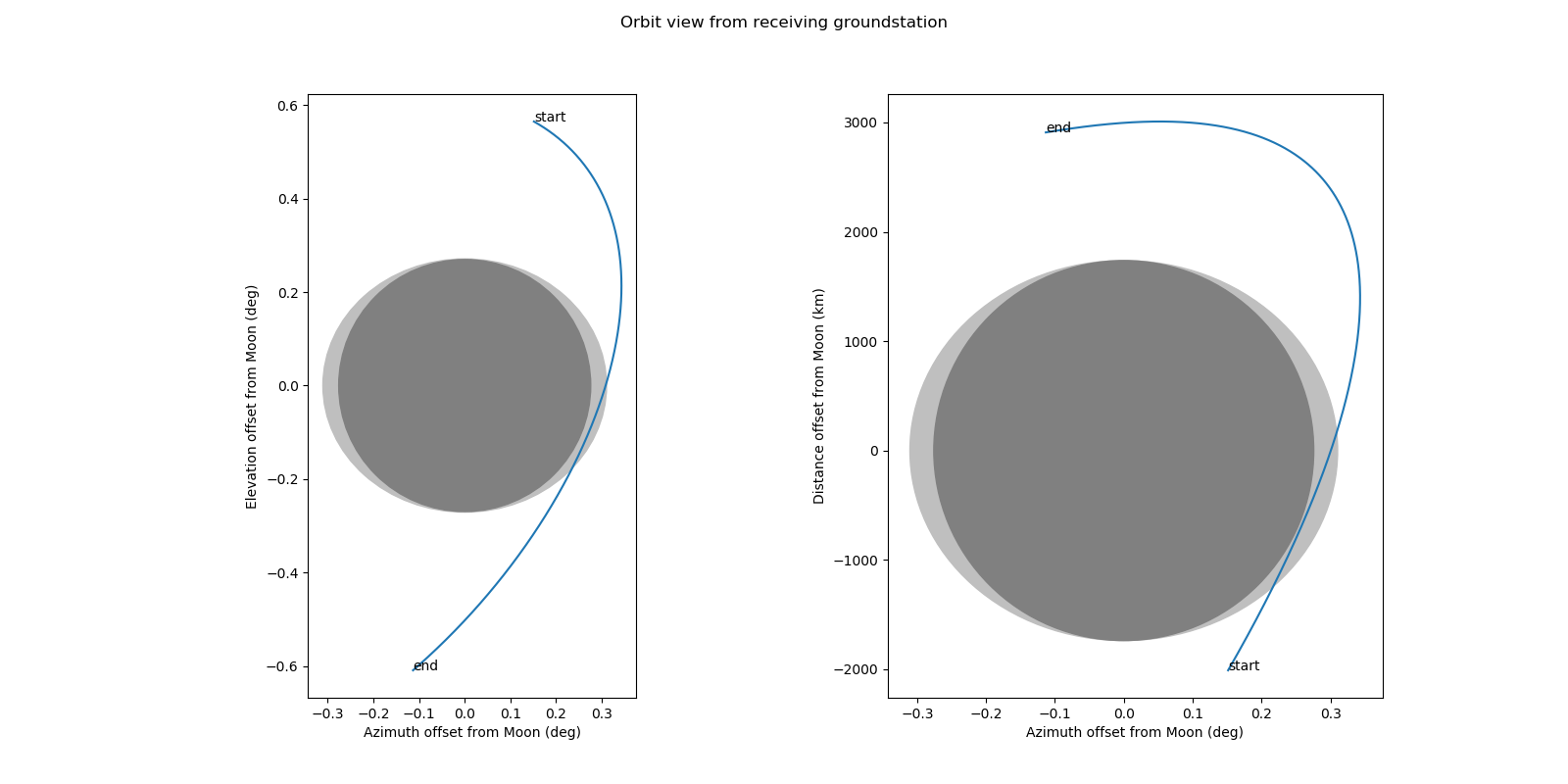
As most of the variation in the size and shape of the ellipse is due to the change in \(\varphi\), we get two ellipses which have the same semi-axis in elevation. The smallest ellipse corresponds to the lowest elevation \(\varphi\) and is shown as a circle due to the aspect ratio of the plot. The largest ellipse corresponds to the highest elevation.