A couple months ago, Andrés Calleja EB4FJV installed a 2.3GHz beacon in his home in Colmenar Viejo, Madrid. The beacon has 2W of power, radiates with an omnidirectional antenna in the vertical polarization, and transmits a tone and CW identification at the frequency 2320.865MHz.
Since Colmenar Viejo is only 10km away from Tres Cantos, where I live, I can receive the beacon with a very strong signal from home. The Madrid-Barajas airport is also quite near (15km to the threshold of runway 18R) and several departure and approach aircraft routes pass nearby, particularly those flying over the Colmenar VOR. Therefore, it is quite easy to see reflections off aircraft when listening to the beacon.
On July 8 I did a recording of the beacon from 10:04 to 11:03 UTC from the countryside just outside Tres Cantos. In this post I will examine the aircraft reflections seen in the recording and match them with ADS-B aircraft position and velocity data obtained from adsbexchange.com. This will show the locations and trajectories which produce reflections strong enough to be detected.
Experiment setup
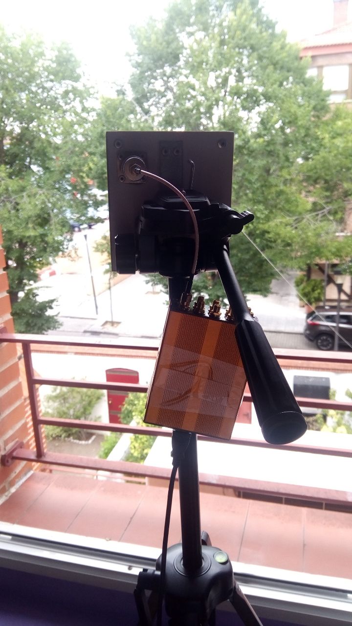
The receiver for this experiment is formed by a LimeSDR connected to a StellaDoradus 9dBi planar 2.4GHz wifi antenna. I chose this antenna rather than a more directive grid parabola because it has a very small form factor and its wide radiation pattern may allow us to receive reflections from unusual directions. The antenna is connected to the LNAH input. The whole receiver setup is mounted on a camera tripod.
The setup can be seen in the picture below, taken at home during testing. The signal in this position is quite strong even though there is not line of sight to the beacon. There are trees just in front of my window and then there are some higher buildings obstructing the direct path.
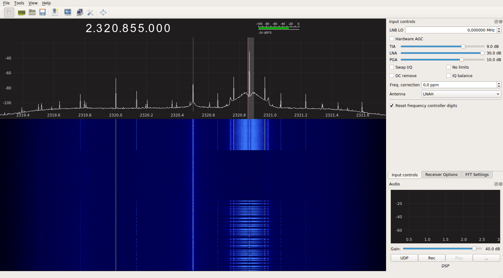
In my usual portable location in the countryside just outside of Tres Cantos I have line of sight to the beacon. The received signal is extremely strong. In the figure below, reciprocal mixing from the local oscillator of the LimeSDR can be seen. Thus with this setup the limiting factor for receiving weak reflections is the dynamic range of the LimeSDR.
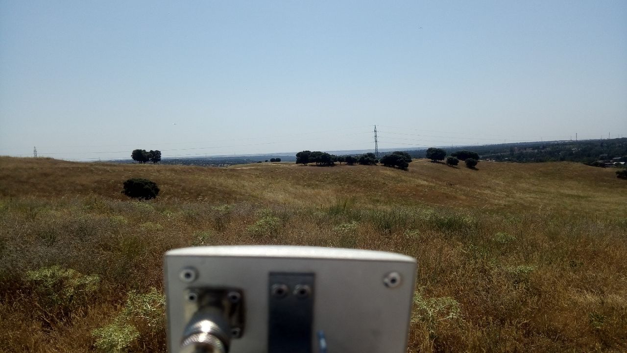
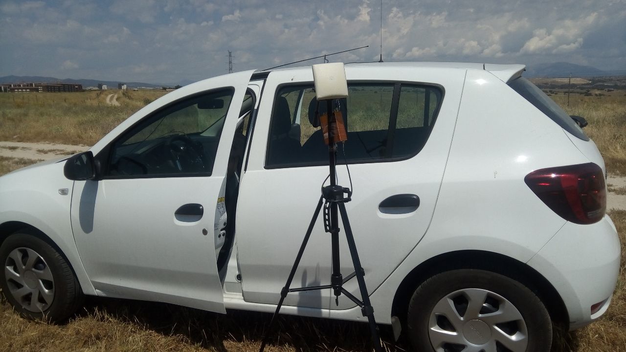
After experimenting for some time in this location with different directions and positions for the receiver, I decided to place the antenna aiming directly towards Barajas, using my car as a makeshift shield for the direct path from the beacon. This is good because I aim the antenna away from the beacon and my car also reduces the direct signal a little. This can be seen in the two pictures below. Note the airplane in the first picture. It is taking off from runway 36L in Barajas and producing a reflection which can be detected in the receiver (click on the image to view it in full size).
My location was the grid locator IN80do68pw (or 40.62045ºN, 3.69466640ºW). The antenna azimuth was set to 120º. At 10:40 UTC I changed the azimuth to 80º, though this did not produce any noticeable difference in the reflections observed.
Recording results
The recording was made in GQRX by recording the audio output in SSB mode with a wide filter. The recording can be downloaded here (738MB). The WAV recording was processed with the script waterfall_13cm.py to produce waterfall data that was saved to an npz file. The resolution of the waterfall data is 11.7Hz or 0.43s per pixel.
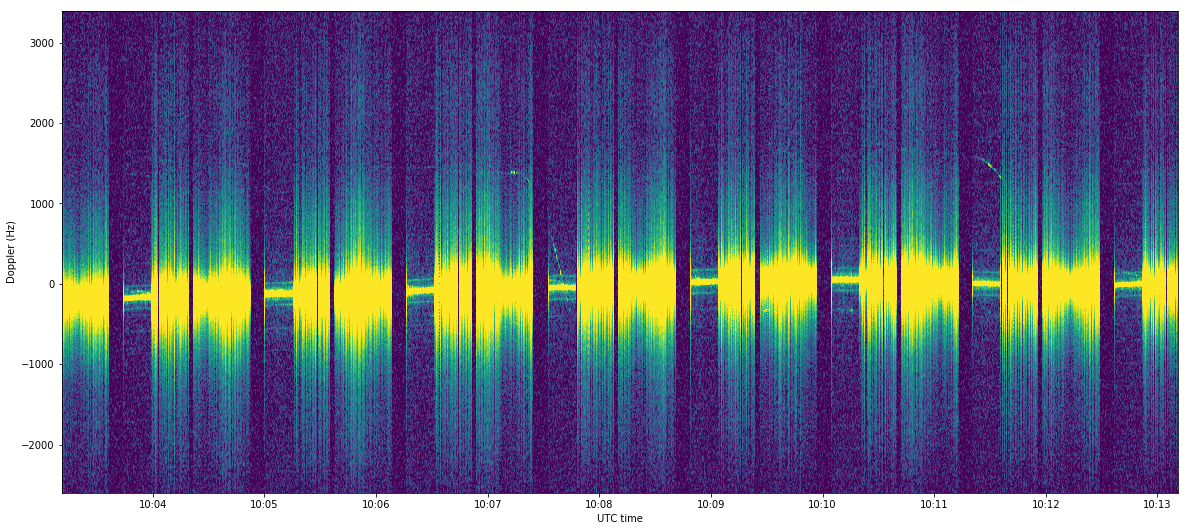
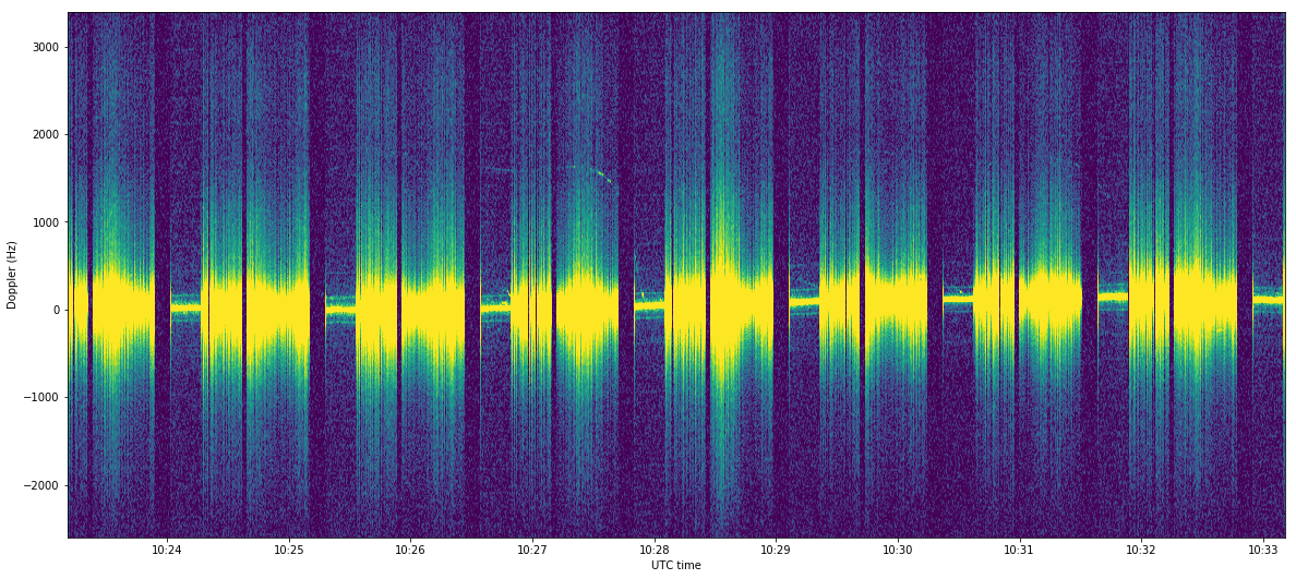
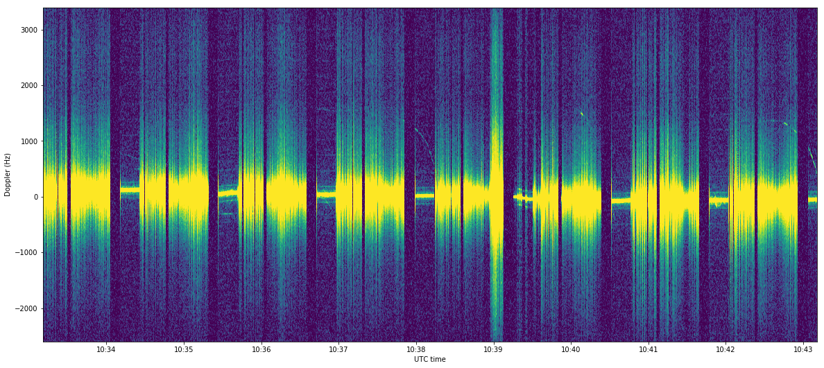
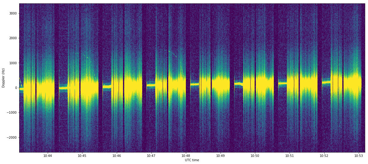
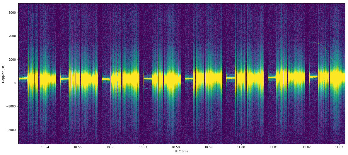
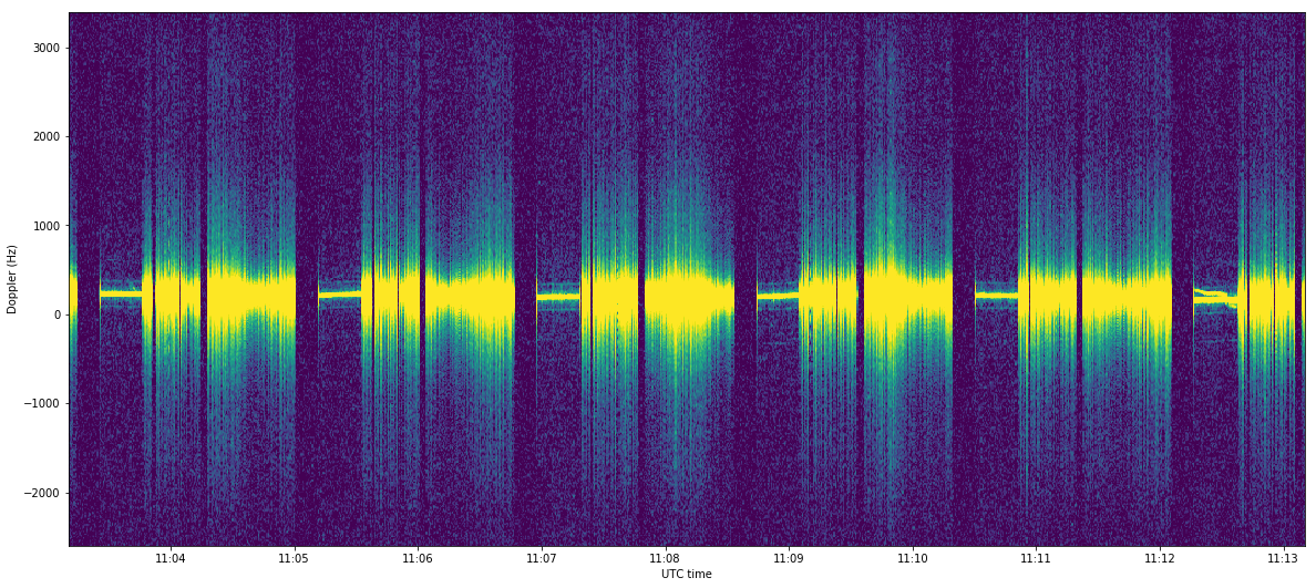
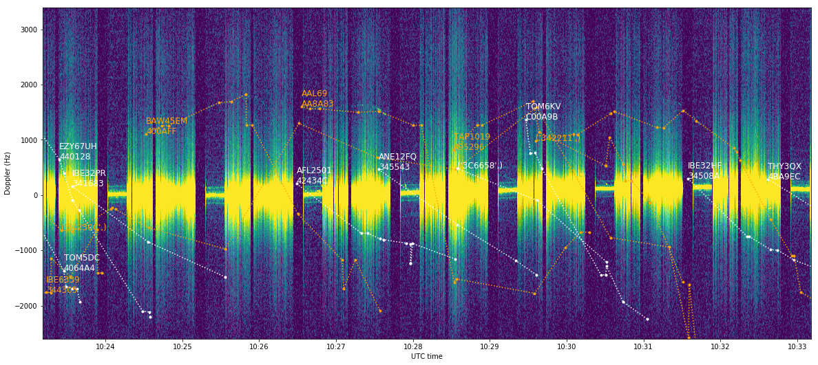
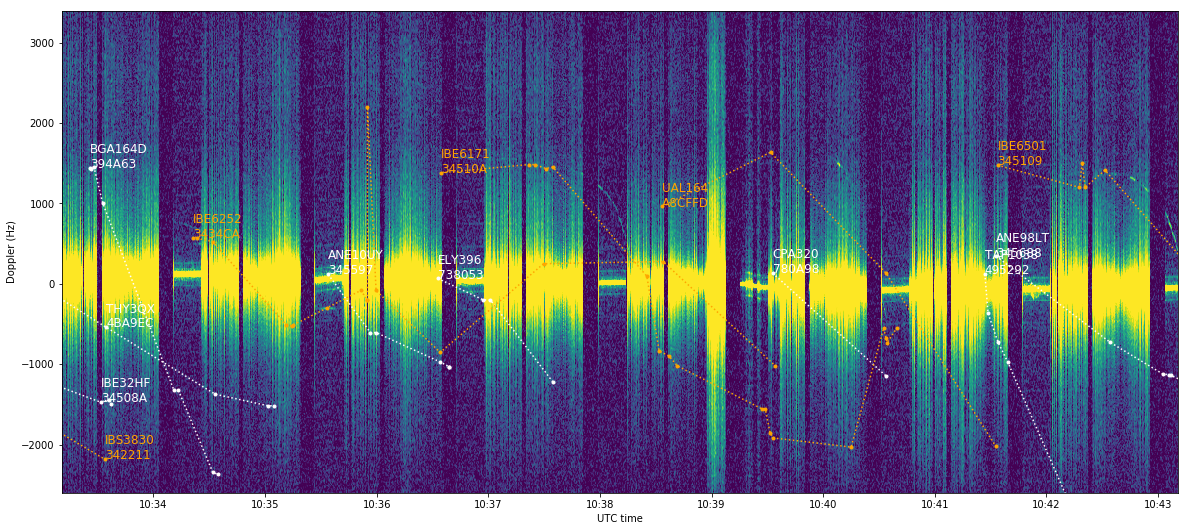
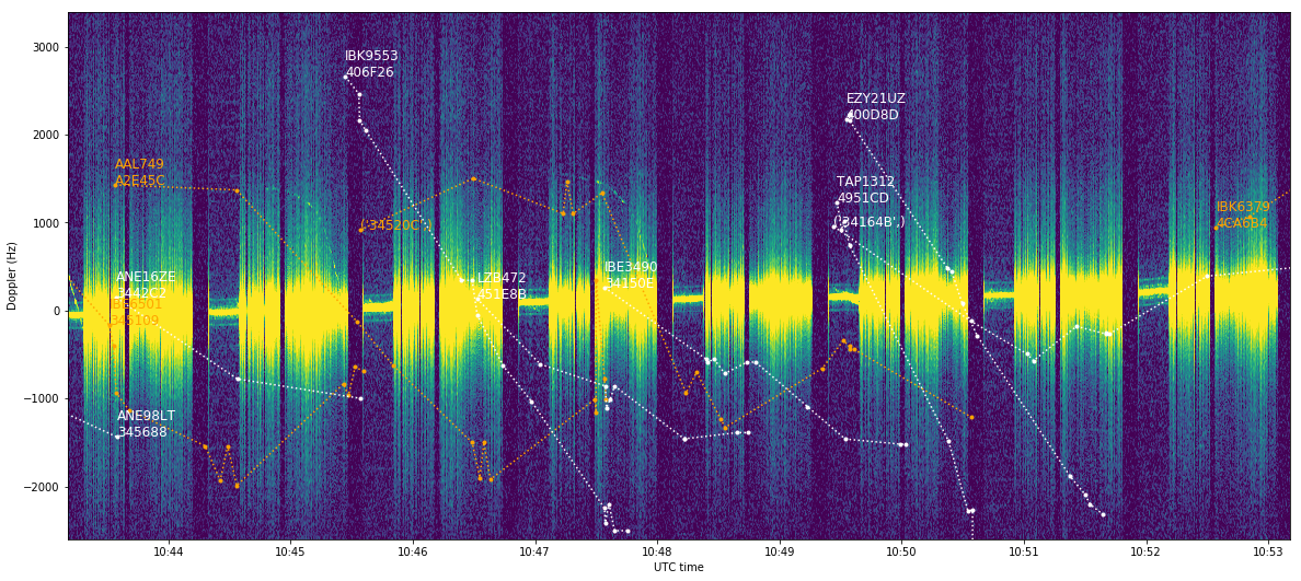
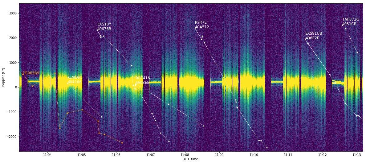
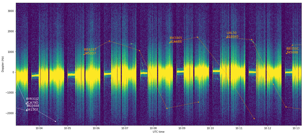
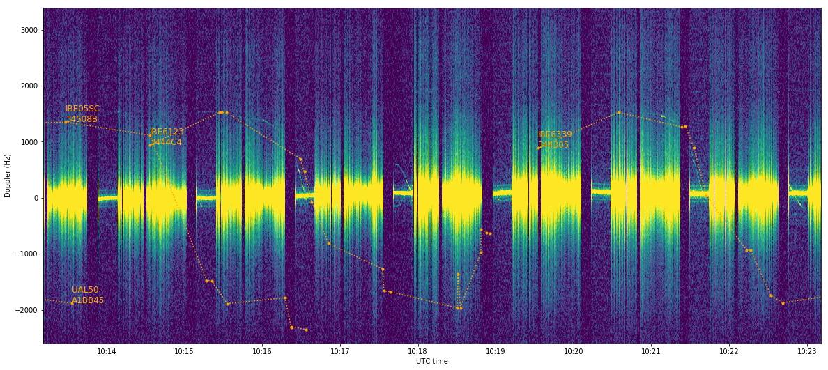
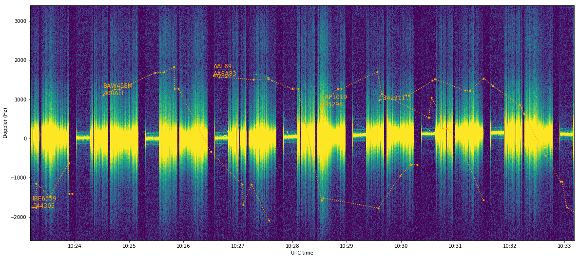
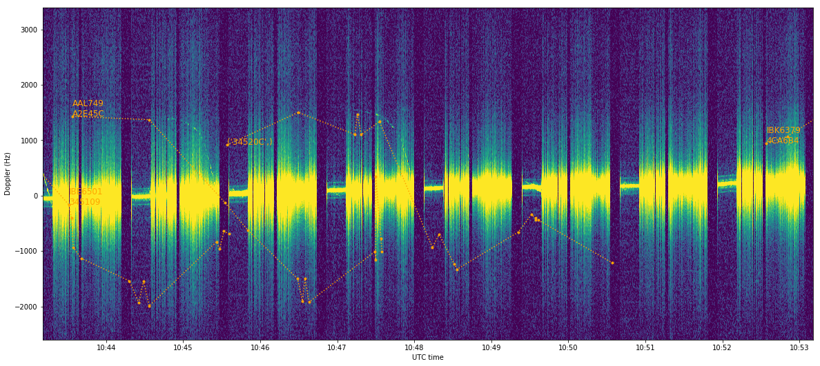
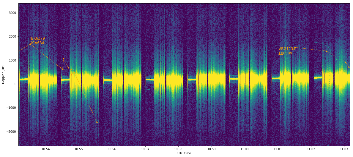
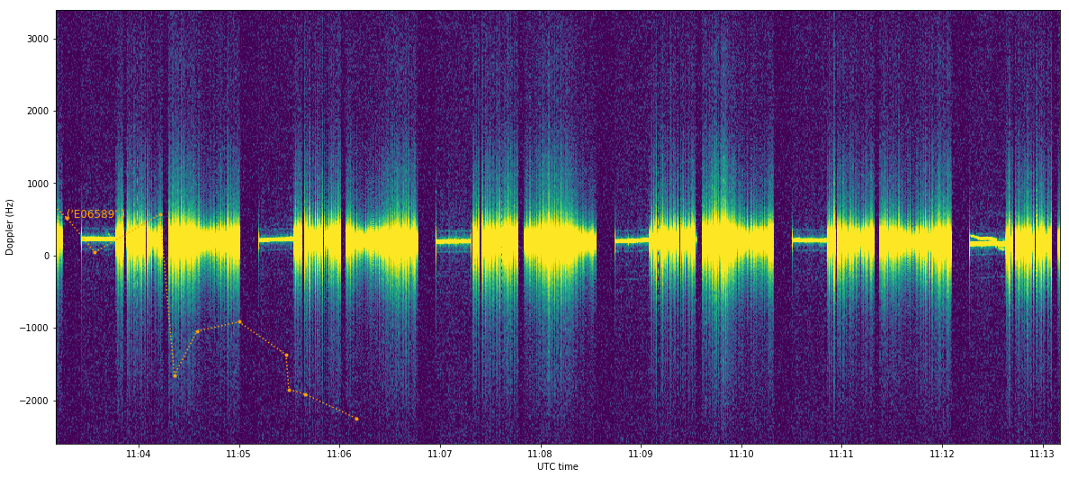
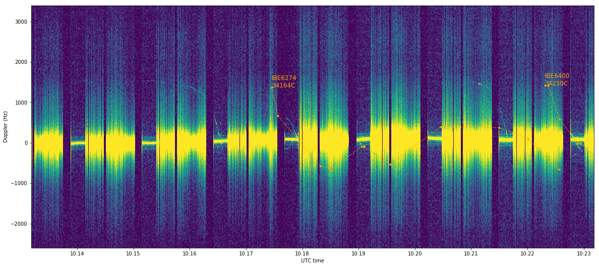
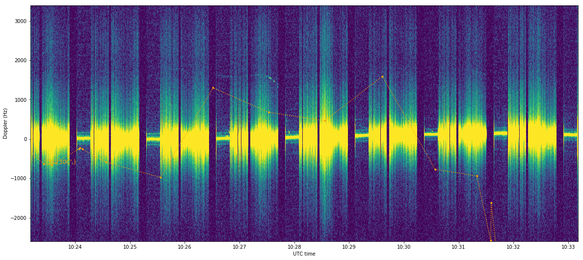
The waterfall can be seen below. It is divided in chunks of 10 minutes for easier visibility. Several aircraft scatter traces are visible, especially with positive Dopplers. Near the end of the last chunk there is something curious: a strong reflection that was produced by a car driving over a nearby dirt road (from several 10s of metres to a hundred metres away). I find it surprising that the reflection is so strong. This opens up the possibility for other experiments. Maybe passive radar traffic monitoring.

ADS-B data
The ADS-B data I have used has been downloaded from the historical data archive of adsbexchange.com. I have made the recommended donation of 0.15 USD per GB to help to cover bandwidth costs. The data is downloaded as a zip file per day. Each of these zip files contains a JSON file per minute with the ADS-B data. The format of the JSON data can be seen here.
The JSON data is loaded in Python using the json library. Unfortunately the JSON data has a few occasional quirks (such as extra commas in lists), so there is some string processing that needs to be done before the json library can accept all files as valid JSON.
Since loading the JSON files is quite slow, once the data is loaded and filtred by geographic location, it is save to a pickled file to load it faster in future executions.
The pymap3d library is used for coordinate transformations. Doppler is calculated in ECEF coordinates. For plotting maps, Cartopy is used together with OpenStreetMap.
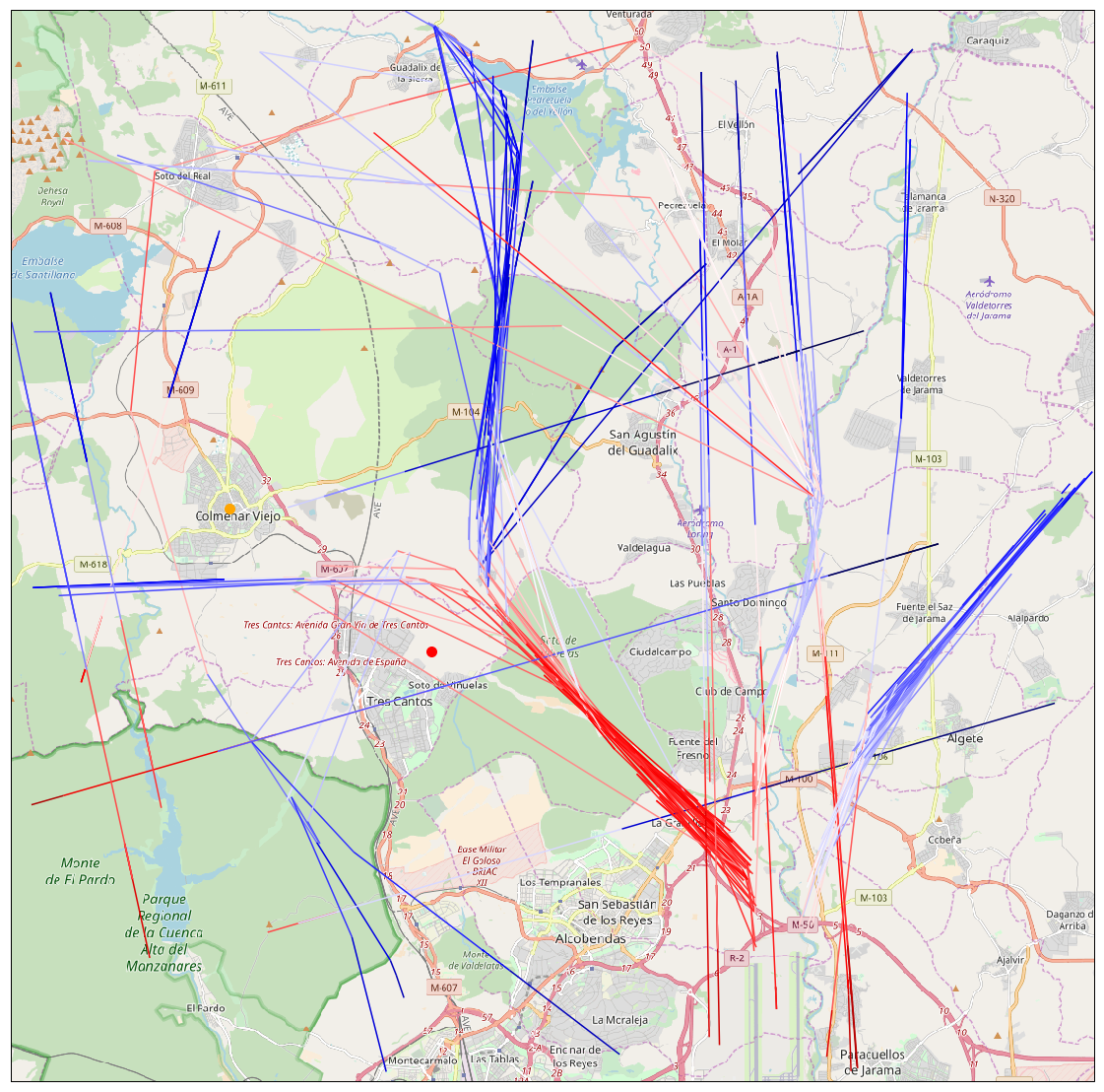
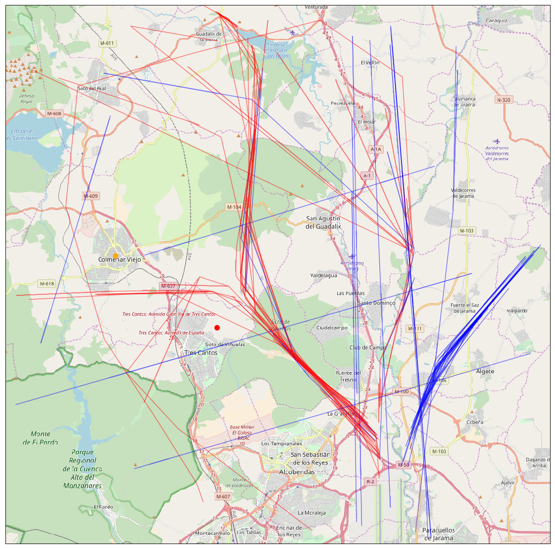
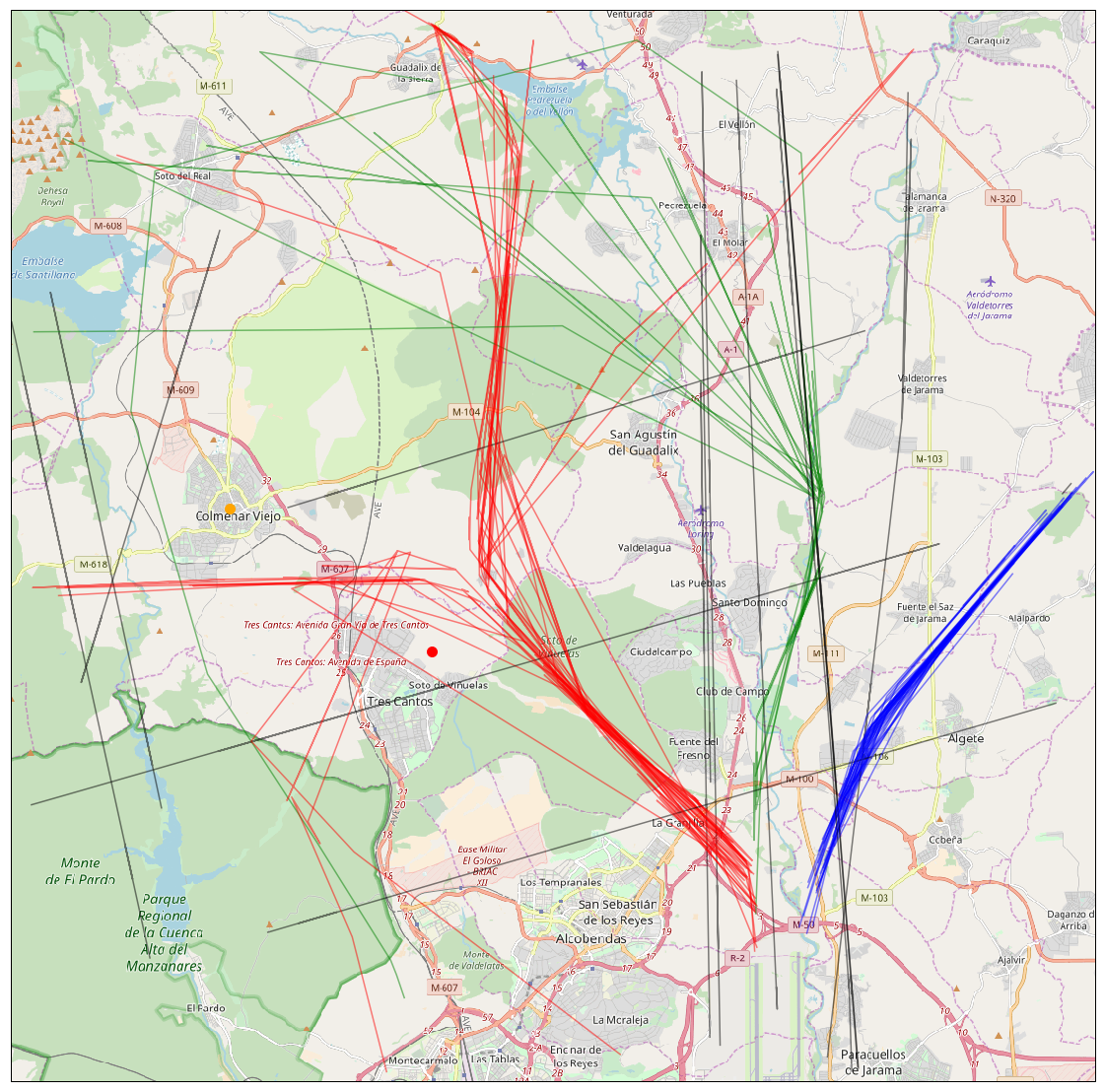
The figure below shows the tracks of all airplanes passing through the zone of the recording between 10:00 and 12:00 UTC. The tracks are coloured by Doppler, with red representing positive Doppler and blue representing negative Doppler. Most of the aircraft that appear in the map are taking off from Barajas’ runways 36L and 36R, since Barajas was in its usual north configuration (takeoff runways 36L and 36R, landing runways 32L and 32R).
The location of the beacon is shown with an orange circle, while the location of my receiver is shown with a red circle.
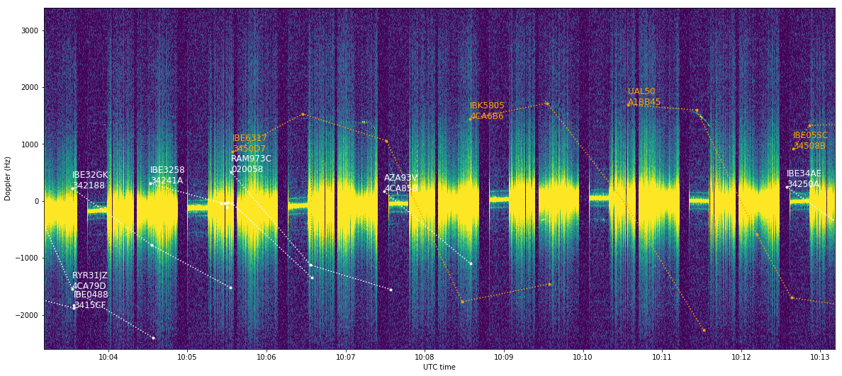
The Doppler traces for each aircraft can now be superimposed on the waterfall to match the reflections with each aircraft. This is done in the figures below. Each Doppler trace shows the aircraft callsign and ICAO hex id. I have selected by hand all the aircraft that produced a reflection of the 2.3GHz beacon and marked their trace in orange. The trace of aircraft which do not produce an observable reflection is marked in white.


Since we have now selected by hand which aircraft have produced a reflection and which haven’t, we can plot again the map of aircraft, marking in red the aircraft which produced a reflection and in blue those who didn’t. This is done in the figure below.
We see that how likely is an aircraft to produce a reflection obviously depends a lot on the route that the aircraft has taken. This leads us to study the aircraft routes more in detail.
Departures from Barajas
Most of the aircraft that appear in the map are departing from runways 36L and 36R from the LEMD (Madrid-Barajas) airport. The route that these aircraft fly is called a Standard Instrument Departure, or SID. The information about the SIDs for a certain airport can be obtained in the relevant AIP (Aeronautical Information Publication). The AIP for Spanish airports can be found online at ENAIRE.
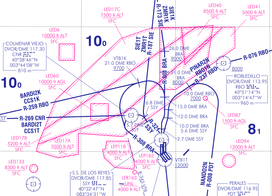
Daytime SIDs for runway 36L are shown in the figure below. They are identified the name of the final fix, a number with the revision of the SID, and a letter indicating the initial route. Currently, they are BARDI2K, BARDI2T, CCS1K, CCS1T, NANDO2N, PINAR2N, RBO1N, SIE1K, SIE1T, VTB1K, VTB1T, ZMR1K and ZMR1T.
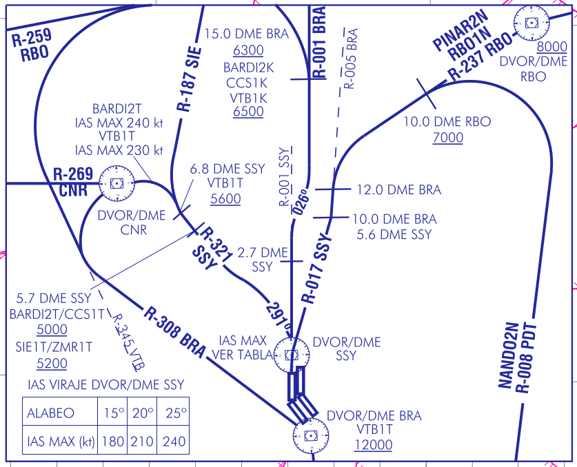
The figure below shows in more detail the initial routes. Aircraft departing on K climb runway heading direct to SSY VOR, then via SSY R-001 to SSY DME 2.7, then turn right to 026º to intercept and follow BRA R-001. Aircraft departing on T climb runway heading direct to SSY VOR, then turn left to 291º to intercept and follow SSY R-321 to SSY DME 5.7 (or 6.8 for VTB1T). Then they turn either left or right depending on the route. Aircraft departing on N climb runway heading direct to SSY VOR, then via SSY R-017 to SSY DME 5.6, then turn right to intercept BRA R-005 to BRA DME 12.
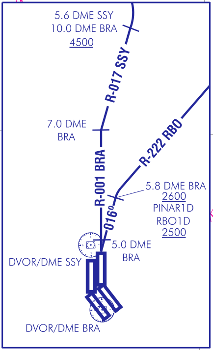
Daytime SIDs for runway 36R are shown in the figure below. Currently they are BARDI5W, CCS4W, NANDO1D, PINAR1D, RBO1D, SIE2W, VTB1D, ZMR2W.
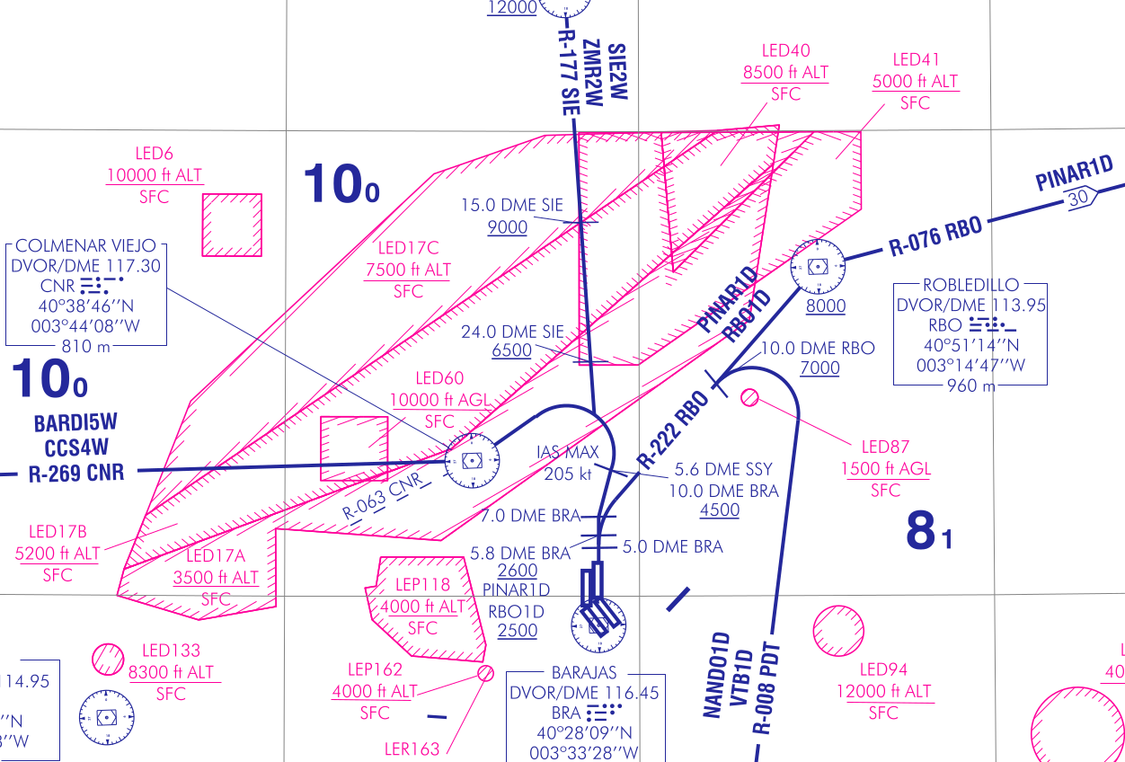
The figure below shows the details of the initial routes. Aircraft departing on W climb runway heading to BRA DME 5, then via BRA R-001 to BRA DME 7, then right to intercept and follow SSY R-017. Aircraft departing on D climb heading 016º to BRA DME 5.8 to intercept and follow RBO R-222.
The next step in our study is to classify the aircraft according to the SID they are flying. The algorithm used is very simple but effective. For each SID we choose a waypoint and assign to that SID all the aircraft that pass within a certain distance of that waypoint. The algorithm for calculating the distance between the aircraft track and waypoint is also simplistic: only positions in the JSON data are considered, rather then interpolating between them. Even though the algorithm is simple, it is able to classify all the aircraft without any mistakes.
The results of the classification are shown below. Each SID is shown in a different colour. Aircraft not flying any SID are shown in black. These are aircraft in cruise flight, most of them flying along the high level routes UN865 and UN870. We are not concerned with them, since none of them have produced any visible reflections. We observe that, from all possible SIDs, only K, T and D are in use. It makes sense not to use N and W in order to keep the traffic for each runway well separated: aircraft departing runway 36L use heading 321º or runway heading, while aircraft departing runway 36R use heading 016º.
Reflections per SID
Now that we have a classification for the SID flowm by each aircraft, we can compute the fraction of the aircraft on each SID that produce a reflection. It turns out that 89% of the aircraft flying T produce a reflection, while 75% of the aircraft flying K produce a reflection. No aircraft flying D produce a reflection. This makes sense, since T takes the aircraft very near the receiver and beacon (indeed I could see the aircraft passing near my receiver), while D takes them away from the receiver and beacon.
Now we study which parts of the routes T and K produce the reflections that we see on the waterfall. Below we show the waterfall drawing only with the Doppler traces for those aircraft on a route T. We note two things. First, all the aircraft except the first two, which had already flown away when the recording started, produce a detectable reflection. Second, the shape of the reflection is as follows: it starts quite flat around 1300Hz, lasts for a minute, then crosses fairly quickly towards 0Hz, increasing in strength and disappears just after passing 0Hz.
This means that the reflection can be detected starting shortly after the airplane takes off from runway 36L. The reflection is visible while the aircraft climbs on SSY R-321. In this part of the route the reflection is backscatter: the receiver is almost inside the line segment joining the 2.3GHz beacon and the aircraft. The receiver’s antenna is pointing directly towards the aircraft. After crossing 0Hz, the airplane turns and flies away from the receiver. It is now on the back of the beam of the receiver, so the reflection disappears quickly.

The waterfalls below show the Doppler traces of aircraft climbing on K. We see that the reflections are only visible for a brief period of time, when the Doppler crosses through 0Hz. This happens when the aircraft has passed SSY DME 2.7 and turns right to heading 026º. In this situation the aircraft is centred on the receiver’s antenna beam, in a good backscatter position, and in the point of its track that is nearest to the receiver.


Closing remarks
In this post we have seen that it is not difficult to receive aircraft scatter in the microwave bands, given an appropriate transmitter and air traffic. This is well known by the Amateur radio community, where people routinely observe aircraft scatter in the VHF, UHF and microwave bands, and even use it for communication. There is a lot of material reporting different situations of aircraft scatter. However, I had never seen a study where the aircraft scatter Doppler traces are matched against aircraft position and velocity data in such a detailed way as it is done in this post.
In these days, ADS-B is a very accessible way of obtaining aircraft position and velocity data. There are several online sources such as adsbexchange.com where it can be streamed in real-time or downloaded for later analysis. Alternatively, it is also possible to receive the ADS-B transmissions at 1090Mhz directly at the aircraft scatter receiver’s location.
The figures shown in this plot have been made in this Jupyter notebook. I have included the supporting data (npz waterfall file and pickled ADS-B JSON data) in the github repository so that interested people can run the notebook again. Hopefully this notebook may serve as the starting point for someone doing its own experiments that require processing and plotting ADS-B data.
In an attempt to get the Amateur radio community interested in topics such as air traffic and air traffic control, I have included an in-depth discussion about the SIDs used at Madrid-Barajas. Of course there are many more air traffic topics relevant to radio than what has appeared here. The reader may want to read and experiment about some of the following: VOR, DME, TACAN, NDB, ILS, primary and secondary radar, ADS-B, mode C transponders, ACARS, VDL, HFDL, Inmarsat AERO, oceanic routes and communications, HF SELCAL, VHF and UHF ATC, METAR and VOLMET, and several more.
Very interesting! Growing up by an airport, some of my earliest radio memories were the local air traffic control frequencies.
Is MSK144 possible at 2.3 GHz, or is there anything that limits the use of that mode on the microwave bands?
It should be possible to use MSK144 in the microwave bands for aircraft scatter (of course not for meteor scatter), but Doppler might be an issue. It would be easy to run some simulations to see how well the decoder holds up against a frequency drift of x Hz/s.
However, I don’t think MSK144 is the best choice for aircraft scatter. It is optimized for short pings (a message repetition lasts only 72ms). In aircraft scatter we usually have at least a few seconds of propagation. Thus, ISCAT (either A, at 1.2s per repetition or B, at 0.6s per repetition) or some of the fast JT9 modes (F is 1.7s/rep, G is 0.85s/rep and H is 0.42s/rep) are much better choices. This probably hold up better against Doppler, too.
Muy interesante y bien elaborado.
Hi, I’m an ATPL student from Tres Cantos, and as well a radio enthusiast, and more regarding aviation. Is all of this rig and “experiment” still up and working? If that’s the case, is there any way that we may communicate via e-mail or something? Thanks and I must say this is a supper interesting post.
Hi Guillermo,
I am not sure if the 2.3GHz beacon in Colmenar Viejo is still running, since it has been a while since I listened to it. Probably it can be put back on the air if it is needed for experiments.
Regarding my side of the experiment, I still have all the equipment I used, and some newer hardware.
You can find my e-mail address at the bottom of this page.
Congratulations for your work!
I have some intention to test aircraft scatter in 432 and 1296 MHz bands. My goal is to compare forward and backward scatter.
Some time ago, I have seen how just a rubber duck antenna, and an FM HT, can receive some far signal under the airway in San Fernando de Henares, only when the plane passes, just listening to the input channel of an analog 432 MHz repeater.
The QSO could not be easily understood. However, the test makes me wonder what would happen with a better antenna.
I was amazed how easy aircraft scatter can be in such excellent conditions!
Thank you for sharing and encouraging these experiments. This is the kind of amateur radio I enjoy!