Having to deal with DSP texts written by engineers, I have sometimes to work a bit to get a good grasp of the concepts, which many times are not explained clearly from their mathematical bases. Often, a formula is just used without much motivation. Lately, I’ve been trying to understand critically damped systems, in the context of PLL loop filters.
The issue is as follows. In a second order filter there is a damping parameter \(\zeta > 0\). The impulse response of the filter is an exponentially decaying sinusoid if \(\zeta < 1\) (underdamped system), a decaying exponential if \(\zeta > 1\) (overdamped system) and something of the form \(C t e^{-\lambda t}\) if \(\zeta = 1\) (critically damped system). Critical damping is desirable in many cases because it maximizes the exponential decay rate of the impulse response. However, many engineering texts just go and choose \(\zeta = \sqrt{2}/2\) without any justification and even call this critical damping. Here I give some motivation starting with the basics and explain what is special about \(\zeta = \sqrt{2}/2\) and why one may want to choose this value in applications.
We start with a linear second order ODE of the form\[\tag{1} a_2y ‘ ‘(t) + a_1y'(t) + a_0 y(t) = f(t).\] This system is known as the damped harmonic oscillator and appears in many physical situations. In particular, it models an RLC circuit, which justifies its appearance in analogue loop filters (and also in their digital counterparts, which work in discrete time).
The Laplace transform of \(y\) is defined as\[Y(s) = \int_0^\infty y(t) e^{-st}\,dt\]provided that this integral converges (usually we restrict ourselves to bounded functions \(y\) and \(\operatorname{Re} s > 0\)). The Laplace transform \(F(s)\) of \(f\) is defined similarly.
Taking Laplace transforms in (1) and assuming that \(y(0) = y'(0) = f(0) = 0\), we obtain\[(a_2 s^2 + a_1 s + a_0)Y(s) = F(s).\]Thus, the transfer function of the system given by (1) is\[H(s) = \frac{Y(s)}{F(s)} = \frac{1}{a_2 s^2 + a_1 s + a_0}.\] In the applications we are interested in, \(a_0\) and \(a_2\) are positive and \(a_1\) is non-negative. By a suitable change of scale we can assume that \(a_2 = a_0 = 1\). We write \(a_1 = 2 \zeta\), so that\[H(s) = \frac{1}{s^2 + 2\zeta s + 1}.\]
The transfer function \(H(s)\) is the Laplace transform of the impulse response of the system, since if \(f\) is a Dirac delta at \(0\), then \(F(s) = 1\), so that \(Y(s) = H(s)\).
The denominator of \(H(s)\) is a second order polynomial. Therefore, the poles of \(H(s)\) are either real or complex conjugates depending on whether the discriminant \(\Delta = 4\zeta^2 – 4\) is positive or negative. We see that for \(\zeta > 1\) (overdamped system), the poles \(\lambda_\pm = -\zeta \pm \sqrt{\zeta^2 – 1}\) are real. This means that the impulse response is a linear combination of \(e^{\lambda_+ t} u(t)\) and \(e^{\lambda_- t} u(t)\), because the Laplace transform of \(e^{\lambda t}u(t)\) is \((s-\lambda)^{-1}\). Here \(u(t) = \chi_{(0,\infty)}(t)\) denotes the step function. The exponential decay rate of the system is \(d = -\lambda_+ = \zeta – \sqrt{\zeta^2 – 1}\). Note that \(d < 1\).
When \(\zeta < 1\) (underdamped system), the poles \(\lambda_\pm = -\zeta \pm i\sqrt{1-\zeta^2}\) are complex conjugate. In this case, the impulse response is again a (real-valued) linear combination of \(e^{\lambda_+ t} u(t)\) and \(e^{\lambda_- t} u(t)\), so it is an exponentially decaying sinusoid. The exponential decay rate is \(d = -\operatorname{Re} \lambda_\pm = -\zeta\). Again, note that \(d < 1\).
In the limiting case \(\zeta = 1\) (critically damped system), the pole \(\lambda = -1\) is double. The impulse response is \(t e^{-t}\), and the exponential decay rate is \(d = 1\). Note that the critically damped case \(\zeta = 1\) maximizes the exponential decay rate.
However, in many applications the exponential decay rate is not the most important parameter to optimize. The plot below, which shows the impulse response for several values of the damping parameter can shed some light into why.
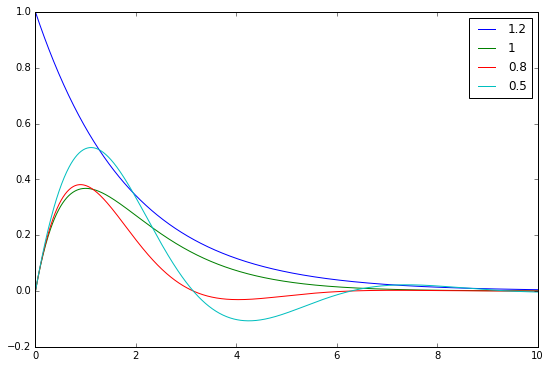
From the four impulse responses plotted, the red one is the most desirable. The blue one, which corresponds to an overerdamped system does not decay fast enough, as we already showed. The exponential decay rate of the green curve, which corresponds to the critically damped case, is the best possible, but the underdamped red curve takes less time to get near zero, because it is an exponentially decaying sinusoid and it has some undershoot. The cyan curve is also underdamped, but it has too much undershoot, since the exponential decay rate is not large enough. Therefore, we see that if the damping factor \(\zeta\) is a bit lower than \(1\) (but not too low), then the undershoot given by the sinusoid plays in our advantage, since it helps bring the response close to zero faster.
Now the obvious question is how low can we set the damping factor before too much undershoot appears. Another way of looking at this problem from a different point of view is studying resonance. When the input \(f(t)\) of the system is a sinusoid of frequency \(\omega\), then \(F(s)\) has poles at \(\pm i\omega\). The Laplace transform of the output of the system \(Y(s) = H(s) F(s)\) has poles at \(\pm i\omega\) and \(\lambda_\pm\). The poles at \(\lambda_\pm\) give terms which decay exponentially, while the poles at \(\pm i\omega\) give sinusoids of frequency \(\omega\) which are still present in the steady state. Thus, when the input is a sinusoid of amplitude \(1\) and frequency \(\omega\), the steady state output is a sinusoid of amplitude \(|H(i\omega)|\) and frequency \(\omega\), since the residue of \(Y(s)\) at \(s = \pm i \omega\) equals the residue of \(F(s)\) at \(\pm i \omega\) multiplied by \(H(i\omega)\). Therefore, the frequency response of the system is given by \(|H(i\omega)|\).
We now compute\[|H(i\omega)|^2 = \frac{1}{\omega^4 + (4\zeta^2 – 2)\omega^2 + 1}.\] Using the substitutions \(\xi = \omega^2\) and \(\gamma = 4\zeta^2 – 2\), we see that the denominator equals the quadratic function \(\xi^2 + \gamma \xi + 1\). The minimum of this quadratic function is at \(\xi = -\gamma/2\). This means that when \(\gamma \geq 0\) the frequency response \(|H(i\omega)|\) is monotone decreasing in \(\omega\). In fact, this system is a low pass filter, so this is not surprising. When \(\gamma < 0\), the frequency response has a maximum at \(\omega_0 = \sqrt{-\gamma/2}\), and \(|H(i\omega_0)| = \frac{1}{1-\gamma^2/4}\). This means that the system has a resonant frequency at \(\omega_0\), and the gain at the resonant frequency is greater than unity. This is undesirable, so we impose \(\gamma \geq 0\). The limiting case \(\gamma = 0\) gives a damping factor of \(\zeta = \sqrt{2}/2\). This is the lowest we can set the damping factor before getting resonance.
The figure below shows the frequency response for different values of the damping factor \(\zeta\). This shows that the system is a low pass filter and it also shows clearly the resonance when \(\zeta < \sqrt{2}/2\).
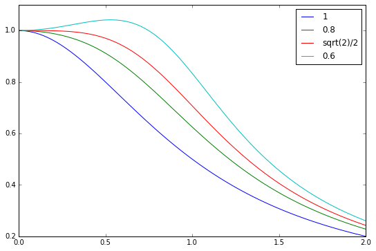
The bandwidth of the low pass filter is defined as the frequency \(\omega\) at which \(|H(i\omega)|^2 = 1/2\). In the case when \(\zeta = \sqrt{2}/2\), a simple calculation using \(|H(i\omega)|^2 = 1/(w^4 + 1)\) shows that the bandwidth is \(1\).