Using band-edge filters for carrier frequency recovery with an FLL is an interesting technique that has been studied by fred harris and others. Usually this technique is presented for root-raised cosine waveforms, and in this post I will limit myself to this case. The intuitive idea of a band-edge FLL is to use two filters to measure the power in the band edges of the signal (the portion of the spectrum where the RRC frequency response rolls off). If there is zero frequency error, the powers will be equal. If there is some frequency error, the signal will have more “mass” in one of the two filters, so the power difference can be used as an error discriminant to drive an FLL.
The band-edge FLL is presented briefly in Section 13.4.2 of fred harris’ Multirate Signal Processing for Communication Systems book. Additionally, fred also gave a talk at GRCon 2017 that was mainly focused on how band-edge filters can also be used for symbol timing recovery, but the talk also goes through the basics of using them for carrier frequency recovery. Some papers that are referenced in this talk are fred harris, Elettra Venosa, Xiaofei Chen, Chris Dick, Band Edge Filters Perform Non Data-Aided Carrier and Timing Synchronization of Software Defined Radio QAM Receivers and fred harris, Band Edge Filters: Characteristics and Performance in Carrier and Symbol Synchronization.
Recently I was looking into band-edge FLLs and noticed some problems with the implementation of the FLL Band-Edge block in GNU Radio. In this post I go through a self-contained analysis of some of the relevant math. The post is in part intended as background information for a pull request to get these problems fixed, but it can also be useful as a guideline for implementing a band-edge FLL outside of GNU Radio.
Band-edge filters
The main idea of the band-edge filters is that the maximum-likelihood estimator for frequency error is given by running the received signal through a matched filter \(g_{MF}(t)\) and through a filter \(g_{FMF}(t)\) whose frequency response is the derivative with respect to frequency of the matched filter frequency response, so that the frequency response of \(g_{FMF}(t)\) is \(G_{FMF}(\omega) = \frac{d}{d\omega}G_{MF} (\omega)\), where \(G_{MF}(\omega)\) denotes the frequency response of \(g_{MF}(t)\), and then taking the real part of the complex conjugate product:\[\operatorname{Re}\left(\int_{-\infty}^{+\infty} g_{MF}(s) y(t – s)\,ds \cdot \overline{\int_{-\infty}^{+\infty} g_{FMF}(s) y(t – s)\,ds}\right),\]where \(y(t)\) denotes the received complex baseband waveform.
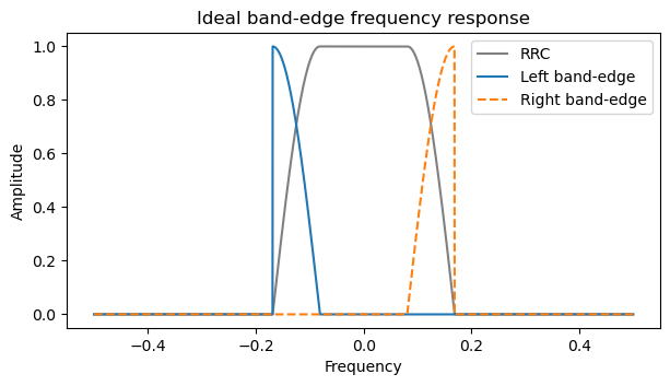
For an RRC waveform, \(G_{FMF}\) is only nonzero in the band-edges, which are the roll-off regions of the RRC frequency response. This is best explained graphically by the following plot, which shows an RRC frequency response and the corresponding band-edges. If we denote these band-edge filters by \(g_{L}(t)\) and \(g_{R}(t)\) for the left band-edge and right-band edge respectively, then \(g_{FMF} = g_{L} – g_{R}\). The plot corresponds to an RRC waveform with 4 samples/symbol and 0.35 roll-off. Note that the band-edge filters are not exactly the derivative of the RRC frequency response. They are scaled to have a maximum value of one, which is common, and simplifies some calculations.
Something that fred harris stresses is that the above expression is the maximum-likelihood estimator, but its variance is often too high to be useful in practice. Instead, he proposes to define filters \(g_C(t) = g_{L}(t) + g_{R}(t)\) and \(g_S(t) = g_{L}(t) – g_{R}(t) = g_{FMF}(t)\) and to use\[\operatorname{Re}\left(\int_{-\infty}^{+\infty} g_C(s) y(t – s)\,ds \cdot \overline{\int_{-\infty}^{+\infty} g_S(s) y(t – s)\,ds}\right)\]as a frequency error estimator that has much lower variance. Note that this expression can be rewritten as\[\left|\int_{-\infty}^{+\infty} g_L(s) y(t – s)\,ds\right|^2 – \left|\int_{-\infty}^{+\infty} g_R(s) y(t – s)\,ds\right|^2,\]which is just the power difference of the two band edges. This is the frequency estimator that I will be using in the rest of this post.
FIR construction of band-edge filters
In the case of an RRC waveform, the roll-off region is a quarter-sine wave (the part of the sine function going from 0 to \(\pi/2\)). Its derivative is also a quarter-sine wave (or better said, a quarter-cosine wave), so that gives the shape of the ideal band-edge filter. However, the frequency response of such an ideal filter jumps immediately from zero to one, because the derivative of the RRC frequency response is not continuous. Therefore, this ideal filter is not realizable as an FIR filter.
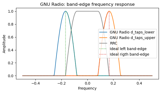
An idea by fred harris is to extend the quarter-sine to a half-sine that is continuous. The time-domain expression for a frequency-domain half-sine can be easily computed as the sum of two sinc functions. This time-domain response can be trimmed to a finite number of coefficients in order to obtain an FIR filter. This technique is explained in this paper, and it is what GNU Radio uses in the FLL Band-Edge block. The frequency response of these band-edge filters is compared below to the ideal band-edge filters.
The drawback of this filter construction is that the band-edge filters have twice more noise bandwidth than they need to have, which degrades the SNR somewhat. More importantly, the increased bandwidth of these filters allows adjacent-channel interference to pass through the filter and affect the frequency discriminator output. For correct operation, a guardband between channels that is at least as large as the roll-off is required. On the other hand, the advantage of this construction is that it is very simple.
Remez design of band-edge filters
An alternative idea to design the band-edge filters is to use the Remez algorithm to obtain an FIR filter that approximates the desired ideal band-edge shape. The Remez algorithm can be used to tune and tradeoff several design criteria, such as faster roll-off and stopband rejection. Using the Remez algorithm to design a band-edge filter is not completely straightforward, because the Remez algorithm can design filters which have either an even or odd frequency response. The band-edge filter has neither. For instance, the right band-edge has a frequency response that is zero for all negative frequencies.
The trick to designing the band-edge filters with the Remez algorithm is to design a filter with even symmetry, which corresponds to the sum of the band-edges, and a filter with odd symmetry, which corresponds to the difference of the band-edges (and hence has purely imaginary coefficients). The right band-edge can be obtained by adding these two filters, so that the left band-edge cancels out. The result is not perfect, because the frequency response of the two filters at negative frequencies is not exactly opposite, so the cancellation is not exact. But it is often close enough.
As an example, let us compare the fred harris / GNU Radio and Remez filter designs for a 4 samples/symbol 0.35 roll-off RRC waveform using 64-tap filters, which is about the smallest reasonable filter size for this kind of waveform.
For the Remez design I am using pm-remez. The design is done by prescribing the following responses:
- Between DC and the start of the roll-off region, response of 0
- In the roll-off region, response following the ideal band-edge
- Between some frequency after the end of the roll-off region and the Nyquist frequency, response of 0
Note that there is a region immediately above the end of the roll-off region in which the frequency response is left unconstrained. This is done so that the filter can transition smoothly between a frequency response of one at the end of the roll-off region, and a frequency response of zero in the stopband.
The parameters that can be tuned in the Remez design are the weights and the width of the transition region. In this case I have experimented and chosen a transition region width which is 37.5% of the roll-off region width. I have set the weights in the two stopbands equal to twice the weight in the roll-off.
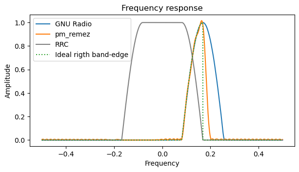
The following compares the GNU Radio and the Remez band-edge filters. The Remez filter goes to zero more quickly at the end of the roll-off, but it has more ripple.
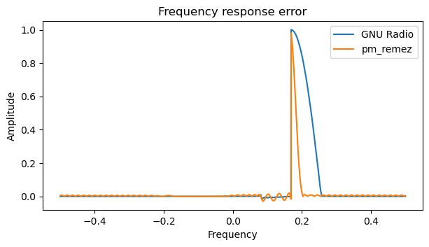
The error of the two filters with respect to the ideal band-edge response also shows quite clearly the increased ripple of the Remez design, in particular in the roll-off region, where the Remez weight is smaller.
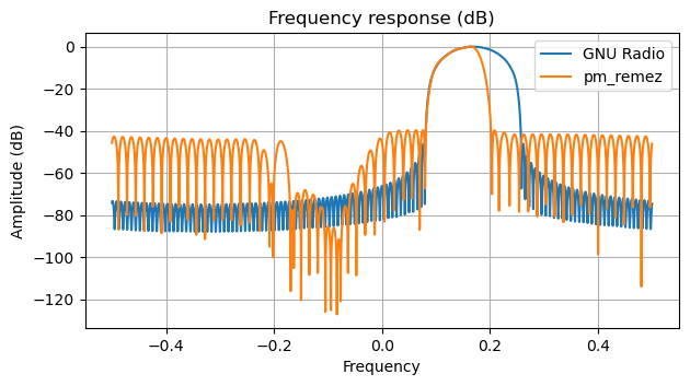
Finally, the frequency response on a dB scale shows that the fred harris / GNU Radio design decays quite rapidly, and the stopband ripple is characteristic of truncating a sinc function, while the Remez design has -40 dB of stopband ripple in most of the passband.
Which of the two filters is preferable depends on considerations about each particular use case, such as whether adjacent-channel interference can be present. The advantage of the Remez design is that it can be tuned to different use cases, while the GNU Radio filter does not have any adjustable parameters.
Discriminant gain
To design the FLL loop coefficients correctly, it is essential to know the discriminant gain. This is a constant that relates the value at the output of the discriminant, which is the difference in powers of the band-edge filters and has arbitrary units of power, with the estimated frequency error, which has units of Hz or of normalized frequency (cycles/sample). More precisely, the discriminant has a transfer function \(K(f)\) that gives the expected value of the discriminant output for a frequency error \(f\). The discriminant gain that we want to find is \(K'(0)\), which is the slope of the transfer function curve at the equilibrium point of the closed loop.
The discriminant is sensitive to the power of the input signal. In fact, its output is proportional to the power of the input signal. Therefore, it only makes sense to compute the gain for a given fixed input signal power. We compute it for an input signal power of one, with the assumption that the signal will be normalized to this power with an AGC when the FLL is used in practice.
We will be performing power calculations by integrating the frequency responses plotted above. Therefore, the first thing we need to calculate is the power of the input signal, since everything else needs to be divided by this power in order to normalize to input power one. To compute this power, we note that the RRC PSD has a value of 1 in the flat region, which has a length of \((1-\alpha)/T_s\), where \(\alpha\) denotes the roll-off and \(T_s\) is the symbol interval in samples/symbol. The roll-off region amplitude is a quarter-sine. Its power is the square of this, which is a raised-cosine, which has an average of \(1/2\). The length of each roll-off region is \(\alpha/T_s\), so each roll-off region contributes a power of \(\alpha/(2T_s)\). The total signal power is\[P = \frac{1-\alpha}{T_s} + 2\frac{\alpha}{2T_s} = \frac{1}{T_s}.\]
The power at the output of the left band-edge filter with a frequency error of \(f\) can be computed as\[\int_{-1/2}^{1/2} |G_L(w)|^2 G_{MF}(w-f)^2\, dw,\]where \(G_L(w)\) denotes the frequency response of the left band-edge filter and \(G_{MF}(w)\) is the frequency response of the RRC waveform. The expression for the right band-edge filter power is analogous. The derivative of the expression above at \(f = 0\) can be calculated by differentiating under the integral sign as follows\[\begin{split}\left.\frac{d}{df}\right|_{f=0}\int_{-1/2}^{1/2} &|G_L(w)|^2 G_{MF}(w-f)^2\, dw\\ &= -2\int_{-1/2}^{1/2} |G_L(w)|^2 G_{MF}(w)G_{MF}'(w)\, dw\\ &= -2\int_{\frac{-1-\alpha}{2T_s}}^{\frac{-1+\alpha}{2T_s}} |G_L(w)|^2 G_{MF}(w)G_{MF}'(w)\, dw.\end{split}\]The last equality is true because \(G_{MF}'(w)\) vanishes outside of the roll-off region.
We see that regardless of how the FIR filter \(g_L\) has been constructed, the only thing that affects the discriminant gain is its frequency response in the roll-off region. Therefore, we will assume that \(G_L(w)\) follows the ideal band-edge response in the roll-off region, which is approximately true when the filter has been designed in a reasonable way.
For simplicity we can change variables and define \(s = w – \frac{-1-\alpha}{2T_s}\) so that the roll-off region is \(0 \leq s \leq \alpha/T_s\). We have\[\begin{split}|G_L(s)|^2 &= \cos^2\left(\frac{\pi T_s}{2\alpha}s\right),\\ G_{MF}(s) &= \sin\left(\frac{\pi T_s}{2\alpha}s\right), \\ G_{MF}'(s) &= \frac{\pi T_s}{2\alpha}\cos\left(\frac{\pi T_s}{2\alpha}s\right).\end{split}\]So we need to compute\[-\frac{\pi T_s}{\alpha} \int_0^{\frac{\alpha}{T_s}} \cos^3\left(\frac{\pi T_s}{2\alpha}s\right) \sin\left(\frac{\pi T_s}{2\alpha}s\right)\, ds.\]This integral can be evaluated for instance in Wolfram Alpha, giving a result of \(-1/2\).
By symmetry, the corresponding derivative for the right band-edge filter is \(1/2\). The derivative of the power difference of the two filters is the difference of these two values, so it is one. Since we need to normalize by dividing by the signal power \(P\), we see that, when the frequency error \(f\) is expressed in cycles/sample, the discriminant gain of the band-edge frequency detector is \(T_s\), that is, it is equal to the samples/symbol parameter. Note that this discriminant gain is independent of how the FIR band-edge filters are constructed, as long as they match the ideal band-edge response in the roll-off region.
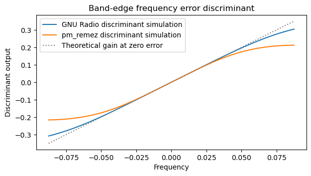
To verify this theoretical calculation, I have done a simulation that estimates the value of \(K(f)\) for the fred harris / GNU Radio FIR filter and for the Remez FIR filter. For this simulation, an RRC waveform at 4 samples/symbol and with 0.35 roll-off is used. The discriminant curves are shown below, compared with a curve with slope equal to \(T_s\). We can see that the slope of the curves matches the theoretical slope at \(f = 0\). Moreover, the discriminants stay almost linear for a reasonably wide frequency range. Something else that can be seen in this plot is that the discriminant with the Remez filter saturates earlier. The reason is that saturation occurs when the frequency errors is so large that one of the band-edges does not contain any signal, and the other band edge is located on the flat part of the RRC spectrum. Since the fred harris band-edge filters are wider in frequency, saturation occurs at a larger frequency error.
FLL loop filter
The main problem with the GNU Radio implementation of the FLL Band-Edge block is that the loop filter is implemented incorrectly. Here I will be using the notation of the paper Controlled-Root Formulation for Digital Phase-Locked Loops, by Stephens and Thomas, which I have already referred to in my post about how to compute PLL filter coefficients. This paper considers discrete-time updates. It denotes by \(\phi_n\) the \(n\)-th phase measurement of the input signal, by \(\hat{\phi}_n\) the \(n\)-th model phase calculated by the loop filter, and by \(\tilde{\phi}_n = \phi_n – \hat{\phi}_n\) the \(n\)-th phase error. The model phase update for a PLL is given by the general formula\[\hat{\dot \phi}_{n+1} T = K_1 \tilde{\phi}_n + K_2 \sum_{i=1}^n \tilde{\phi}_i + K_3 \sum_{i=1}^n \sum_{j=1}^i \tilde{\phi_j} + \cdots,\]where \(T\) is the loop update interval.
An FLL is different from a PLL, because the discriminant measures frequency rather than phase. Therefore, in an FLL loop update only the signal frequency \(\dot \phi_n\) is available. The loop update needs to be written in terms of frequency errors \(\tilde{\dot \phi_i} = \dot \phi_i – \hat{\dot \phi_i}\), and the error must act on the frequency accumulator and higher-order accumulators, rather than directly on the model phase increment as a PLL does. This means that the update is\[\hat{\dot \phi}_{n+1} T = K_1 \sum_{i=1}^n \tilde{\dot \phi}_i + K_2 \sum_{i=1}^n \sum_{j=1}^i \tilde{\dot \phi_j} + \cdots.\]
For clarity, this is better expressed in pseudocode. For a second-order PLL, the loop update is as follows.
frequency += k2 * phase_error;
phase += frequency + k1 * phase_error;
The equivalent loop update for an FLL is however the following.
frequency += k1 * frequency_error;
phase += frequency;
Note that if the measured signal frequency \(\dot \phi_n\) refers to the average frequency over the update interval, or if \(\dot \phi_n\) refers to instantaneous frequency and we apply the continuous update approximation, then \(\dot \phi_n T = \phi_n – \phi_{n-1}\), so the loop update for an FLL can be rewritten as\[\hat{\dot \phi}_{n+1} T = \frac{K_1}{T} (\tilde{\phi}_n – \tilde{\phi}_1) + \frac{K_2}{T} \sum_{i=1}^n (\tilde{\phi}_i – \tilde{\phi}_1) + \cdots.\]This means that, except for the initial phase term \(\tilde{\phi}_1\), which is present because the discriminant is not phase sensitive and so the loop cannot drive the phase error to zero, the FLL looks the same as a PLL with coefficients \(K_j/T\). Therefore, all the considerations and formulas in the paper by Stephen and Thomas about PLLs can be used here.
Since we want to design a loop filter with only one coefficient \(K_1\), as in the pseudocode given above, we use the continuous-update approximation in the paper, which gives\[K_1 = \kappa_1 T = 4 B_L.\]This is the coefficient for a first-order PLL. For an FLL the coefficient needs to be multiplied by \(T\), so we get\[K_1 = 4 B_L T.\]Dimensionally this coefficient makes sense, because it transforms an error in units of frequency into a frequency that is added to the frequency accumulator.
Care needs to be taken to scale \(K_1\) appropriately according to the units which are used. In GNU Radio, the loop model phase uses units of radians, and the frequency accumulator uses units of radians/sample. Above we have computed that the discriminant gain, when the frequency error output is expressed in cycles/sample, is \(T_s\). Therefore, to account for the unit conversion and the discriminant gain, the coefficient \(K_1\) that needs to be employed in an implementation like GNU Radio is\[K_1 = \frac{8 \pi B_L T}{T_s}.\]The user of the FLL is expected to supply the parameter \(B_L T\), which is the normalized loop bandwidth. It can be computed as the product of \(B_L\), which is the loop noise bandwidth in Hz, and \(T\), which is the sampling interval in seconds, since the FLL performs a loop update for every input sample.
GNU Radio legacy loop filter
The loop filter update in the existing GNU Radio code is as follows.
frequency += beta * frequency_error;
phase += frequency + alpha * frequency_error;
The loop coefficients are computed in terms of a bandwidth parameter, which I will denote by \(B\), using the formulas\[\begin{split}\alpha &= \frac{2 \sqrt{2} B}{1 + \sqrt{2} B + B^2},\\ \beta &= \frac{4 B^2}{1 + \sqrt{2} B + B^2}.\end{split}\]As mentioned above, the coefficient \(\alpha\) should be equal to zero, because the FLL should not act directly on the phase increment update. An \(\alpha \neq 0\) only contributes to an increased loop noise. To find an approximate relation between the bandwidth parameter \(B\) in the legacy code and the normalized loop bandwidth \(B_L T\), we can impose \(\beta = K_1\) and solve for \(B_L T\). This gives\[B_L T = \frac{B^2}{1 + \sqrt{2}B + B^2}\cdot \frac{T_s}{2\pi}.\]Note that this is a nonlinear relation, so the legacy bandwidth parameter \(B\) was quite bad in the sense that modifying its value affected the loop bandwidth non linearly.
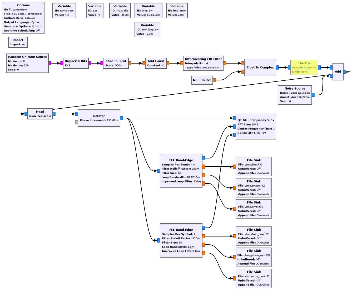
In order to validate these changes, I have set up a comparison of the legacy loop filter and the new loop filter in a GNU Radio simulation. The flowgraph I have used is shown here. A BPSK RRC waveform at 4 samples/symbol with a roll-off of 0.35 is generated. A frequency offset of 10% of the symbol rate is applied, and the signal is sent to two independent FLL Band-Edge blocks. The outputs of these blocks are written to files for analysis.
The first FLL Band-Edge block uses the legacy loop filter with a bandwidth parameter \(B =2 \pi/100\), which is commonly used in examples and unit tests (although the reason for this choice is not clear).
According to the relation given above between \(B_L T\) and \(B\), the corresponding \(B_L T\) would be approximately \(2.3 \cdot 10^{-3}\). However this relation is an approximation, because it does not take into account that the legacy loop filter uses an \(\alpha \neq 0\). Therefore, to adjust \(B_L T\) for the second FLL Band-Edge, which uses the correct loop filter I have described above, I have used \(2.3 \cdot 10^{-3}\) as a starting point, and adjusted it by hand until obtaining a convergence time which is very similar to the one obtained with the legacy loop filter. This has given me a loop bandwidth of \(B_L T = 1.6 \cdot 10^{-3}\).
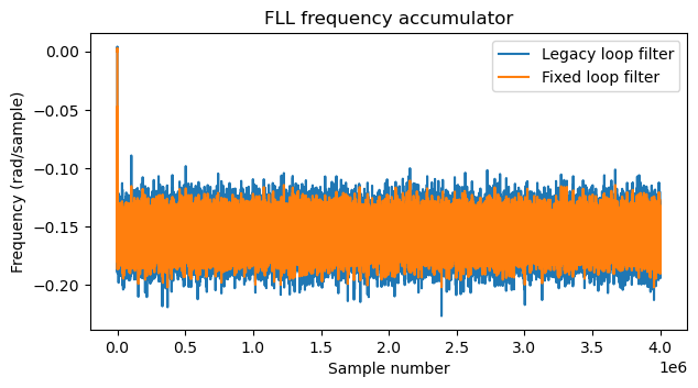
The following plot shows the value of the frequency accumulator for the two FLLs at the beginning of the simulation. We can see that they converge almost at the same time, but already we can see that the fixed loop filter is less noisy.
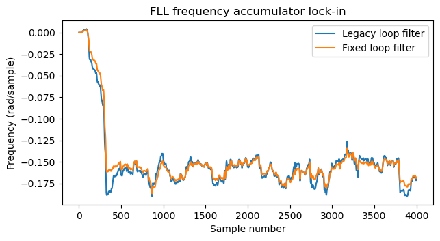
The next plot compares the value of the frequency accumulator in both loop filters. We can also see that the fixed loop filter is less noisy.
Finally, the following plot uses the NCO phase of the FLL to compute frequency as the phase derivative. The legacy loop filter is much more noisy, due to the effects of a nonzero \(\alpha\) acting directly on the phase update.
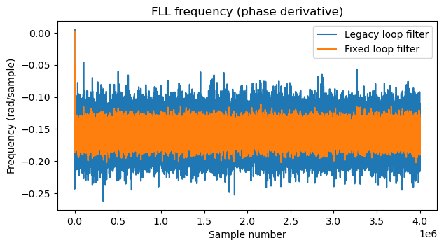
Therefore, we see that the new fixed loop filter is a substantial improvement over the legacy one. When the bandwidth is adjusted to obtain the same convergence time, the loop has much less noise.
Code
The Jupyter notebooks and the GNU Radio flowgraphs used in this post can be found in this repository. The fixed loop filter for the FLL Band-Edge block is to be submitted in a PR to GNU Radio.