Since the end of August I have been working on a new ADS-B receiver application that is intended to outperform existing open source receivers in scenarios with weak signals or message collisions. Now I have reached a point where this software is ready to be published. The name of this project is more1090, and it is a Rust application and library licensed under an Apache 2.0 or MIT license. The receiver operates at 8 Msps IQ and uses FFTs for signal detection. Therefore, it is much more CPU intensive than other ADS-B receivers such as readsb. It will probably not run on your Raspberry Pi (I haven’t tried; maybe there is a hope for the Pi 5 or other modern high-performance ARM boards), but it runs 4 times faster than real-time on a modern x86-64 laptop (the receiver is single-threaded, so the core count doesn’t matter), and it can decode way more messages than readsb.
The more1090 receiver only decodes Mode-S extended squitter replies (DF17 and DF18), which is how ADS-B is transmitted at 1090 MHz. Other receivers such as readsb also attempt to decode other Mode-S reply message types and even Mode-A/C replies. The challenge to decode other Mode-S message types is that only extended squitter and acquisition squitter (one particular use of DF11) are intended to be broadcast messages to be decoded by any receiver. The remaining messages are intended to be replies to an interrogator, to be decoded only by that interrogator. Their CRC is XORed with information only known to the interrogator, such as the ICAO address of the replier or the interrogator identification code. Therefore, it is difficult for another receiver to determine if it has decoded these messages without errors. Because of this, more1090 focuses on decoding extended squitter messages as best as possible and ignoring everything else. It is possible to decode acquisition squitter messages using a similar approach, but these messages only contain the ICAO address of the transmitter, so they are of limited interest, and decoding them is not implemented at the moment.
In addition to the ADS-B receiver, more1090 contains a signal simulator that can generate all types of Mode-S and Mode-A/C replies that appear at 1090 MHz in the real world. This simulator can generate both signal snippets containing a single message, which are useful for benchmarking things such as decode probability at a given CN0, and full scenarios which contain all message types with transmission times following a Poisson process. The full scenarios characterize the receiver performance in more realistic conditions.
At the moment this simulator doesn’t generate TACAN/DME signals. There are a few ground-to-air TACAN channels that are within 4 MHz of 1090 MHz: 125Y, 126Y, 1Y, 2Y, 3Y, 4Y, 5Y, 6Y, 7Y. These channels are used infrequently (an example is the SSY VOR/DME in Madrid, Spain, which transmits on 125Y at 1086 MHz). Additionally, there are also air-to-ground TACAN channels within 4 MHz of 1090 MHz: 62X, 62Y, 63X, 63Y, 64X, 64Y, 65X, 65Y, 66X, 66Y, 67X, 67Y, 68X, 68Y, 69X, 69Y, 70X, 70Y. Real world usage of these channels includes around 100 civilian VOR/DME, VORTAC or DME-only in channel 70X (1094 MHz) and a number of military TACAN in the remaining X channels. These are a potential source of interference to ADS-B and other secondary surveillance radar services at 1090 MHz.
The signal simulator is used for benchmarking the more1090 receiver, both in synthetic conditions (isolated messages at a fixed CN0) and in scenarios which are representative of a typical terrestrial receiver and a typical receiver on a LEO satellite.
In the rest of this post I explain more details about this new ADS-B receiver.
Motivation of receiver techniques
I began working on this project mainly out of disappointment with the quality of existing open source ADS-B receivers. This shouldn’t come as a surprise. In GRCon19, Robin Getz gave a talk with the inconspicuous title Optimizing Radio Settings for Algorithms. In this talk he explained that many open source receivers were quite bad. The main reason for this is that most of them stemmed from forks (or forks of forks) of dump1090, which was made for the RTL-SDR. Therefore, these receivers tend to use a low sample rate (2 Msps and 2.4 Msps are typical), and 8-bit IQ. As we will see below, the main-lobe bandwidth of Mode-S replies is 4 MHz, so 2.4 Msps is clearly insufficient to obtain reasonable results. Robin also explained that “I can see planes” is not proper benchmarking, because even a receiver with huge implementation losses can decode the strongest ADS-B messages. He stressed the need for doing reproducible and correct sensitivity testing. The rest of the talk focused more on how to optimize the configuration of AD936x parts for this particular use case rather than on ADS-B receiver DSP algorithm design (hence the title of the talk).
I started thinking about building a new ADS-B receiver when I noticed that readsb was performing very poorly in scenarios that tended to have weaker messages and many collisions. My initial line of thinking was “why are all open source ADS-B receivers bad?”, but it doesn’t make much sense to ask this question in absolute terms. It makes more sense to ask “what would be better ways of decoding ADS-B?”. This gives us some insight into what is the gap and how much performance these receivers might be missing.
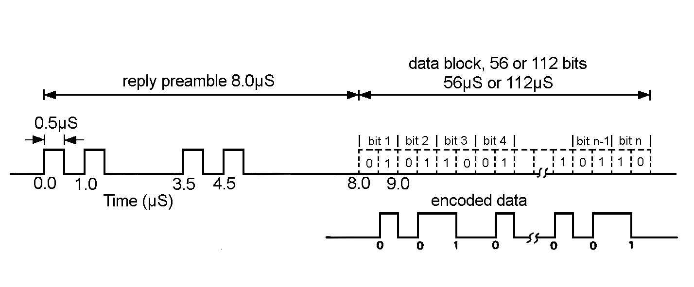
To talk about this in more detail, we need to familiarize ourselves with how ADS-B messages are modulated. Secondary surveillance radar (SSR) Mode-S replies use pulse position modulation with 0.5 usec pulses. Each bit is sent as a 1 usec interval that either has a pulse on the first half to indicate a 1 or a pulse on the second half to indicate a zero. There are short messages, which consist of 56 bits (32 bits of data and 24 bits of CRC) and long messages, which consist of 112 bits (88 bits of data and 24 bits of CRC). ADS-B uses extended squitter messages, which are long messages. Before the message data, there is a preamble that has a duration of 8 usec and contains 4 pulses. These 4 pulses can be interpreted as the bits 11, followed by a gap of one empty bit, then the bits 00, and then a gap of 3 empty bits. The following diagram taken from Wikipedia illustrates the modulation and message structure.
I haven’t looked in much detail into how readsb and similar dump1090 derivatives work, but I imagine they work in the following straightforward way, which is how a traditional analogue receiver would work: The incoming IQ data is run through some simple pulse shape filter that accumulates the energy in each 0.5 usec pulse (at 2 or 2.4 Msps this is basically a no-op, because the pulse duration is one sample). Then there is power detection. Some thresholding decides what is a pulse and what isn’t. The threshold might be adaptive, based on looking at the noise floor power level. The receiver performs pattern matching to find the preamble sequence. Once it finds it, it demodulates the message data by comparing the power in the two possible pulse positions for each bit. This naïve approach is quite similar to what I used to implement a DME receiver, minus the fancy matched filter techniques I used to obtain accurate time-of-arrival estimates. This is good for high-SNR scenarios, but it is far from the best we can do if we are interested in weaker signals.
It is quite clear which elements of this approach are particularly bad. First, the low sample rate is a problem. At 2 or 2.4 Msps we only have one sample per pulse, and the alignment of that sample to the pulse timing is something outside of our control (at 2.4 Msps we have 1.2 samples per pulse, so the alignment changes periodically throughout the message). At only 1-1.2 samples per pulse fractional resampling is not so helpful, because it requires some excess bandwidth to work well. Additionally, we are hugely affected by how the SDR obtained this low sample rate. Since we are discarding roughly half of the signal bandwidth, the shape of the SDR passband has a major effect.
Detecting what is a pulse by thresholding is problematic in busy scenarios, as it is difficult to estimate the noise floor if the channel is busy most of the time. A fixed threshold could be used, but it would need to be tuned specifically for a particular receiver gain and RF environment. Additionally, the preamble detection is quite frail. Especially if there are chances for collisions, there are many cases in which we can miss the preamble, which means that we miss the whole message.
If we think from scratch about how to decode these Mode-S reply messages, the first tasks that the receiver must do are detection and synchronization. When comparing different approaches, it is useful to think in terms of energy: how much energy, from the total energy used to transmit the message, are we using for detection and time and frequency estimation? This way of thinking steers us to techniques that work better for weak signals. For instance, in this case we see that a long Mode-S reply consists of 120 pulses, only 4 of which are in the preamble. This means that if our detection and synchronization strategy uses only the preamble, we are using only 3.3% of the energy that is available.
To come up with a detection system that uses a much larger amount of energy, we first need to answer the following question: are the pulses in a Mode-S reply message coherent? That is, do all the pulses have the same phase, or does each pulse have a random phase? The technical requirements don’t say. Essentially, they allow any kind of horrible RF oscillator as long as it complies with the spectral mask. These might have been a thing in the past, but the current reality is that almost all the Mode-S equipment has solid-state transmitters that generate a coherent sequence of pulses.
Under the assumption that the pulses are coherent, we see that the pulse position modulation is equivalent to residual-carrier phase modulation with Manchester encoded symbols and 50% of the power allocated to the residual carrier and 50% of the power allocated to the data. This is the usual PCM/PM/bi-phase-L modulation used in spacecraft communications. The reason for this equivalence is simply that if we subtract a constant 0.5 (which represents the residual carrier) from the Mode-S message, we get a Manchester encoded waveform with an amplitude of 0.5.
This equivalence tells us a few things that were not so obvious when viewing the message as pulse position modulation. First, it shows us that the power spectral density of Mode-S replies is the same as PCM/PM/bi-phase-L, which is something I’m very familiar with from my work in spacecraft communications. The following shows the spectrum of a recording I made at 1090 MHz to use as an example to develop more1090. Compare this with the spectra in this post about JUICE, for instance.
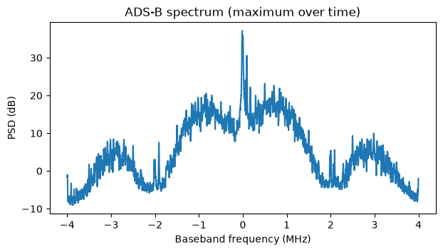
Note that the fact that we can see a strong residual carrier in this 1090 MHz spectrum proves that the transmitters are coherent. If each pulse had a random phase uniformly distributed over the unit circle, then the message would have no DC component on average, and we wouldn’t see a residual carrier in the spectrum.
This equivalence suggests a good way to detect and synchronize to the message. We can use the residual carrier. It contains 50% of the transmitted energy, and it is concentrated in frequency, so it is easy to detect.
Additionally, thinking about this waveform as PCM/PM/bi-phase-L immediately tells us what is the theoretical limit for packet error rate at a given CN0. Taking into account that only 50% of the power is allocated to the data, the BER vs Eb/N0 curve is the same as for BPSK. This also motivates us to do coherent demodulation. The naïve receiver I described above uses noncoherent demodulation by comparing the powers of the two possible pulse positions. As we will see below, this is roughly 1.8 dB worse, and less tolerant to interference from collisions, because coherent demodulation provides some rejection to interference that occurs 90º out of phase with respect to the message.
With this line of reasoning, we can also see that we should mostly ignore the Mode-S preamble. It only has 4 pulses distributed over 8 microseconds, so it has half the energy density of the message payload, and it doesn’t contribute much energy.
The residual carrier can give us reliable message detection, quite accurate frequency and phase synchronization, and a coarse time synchronization (It is inherently coarse because the autocorrelation of the residual carrier is a triangle whose base is 224 usec long. This shows the difference between using an unmodulated carrier for time synchronization versus using a carrier modulated with a pseudorandom sequence). Synchronization is usually the hardest part of decoding, and in this case this is also true.
Once we have synchronized using the residual carrier, the only thing we are missing to attempt coherent demodulation is the symbol alignment and start of message alignment. The message is short enough that we do not need to worry about the symbol clock drifting throughout the message (100 ppm of error over 112 bits is only 0.01 of a bit). It is feasible to do brute force decoding and try all possible alignments, searching for a message that gives a correct CRC check. Technically speaking, the set of all possible alignments is infinite, since the symbol clock phase has a fractional part. However, with an appropriate sample rate we can limit the search to integer sample delays. In this case, a very reasonable sample rate choice is 8 Msps. This gives 4 samples per pulse, which is usually a nice number to work with, as it provides adequate excess bandwidth. As shown in the spectrum above, in 8 MHz we capture the main lobe and the first sidelobe of the Mode-S message modulation, which uses an almost rectangular pulse shape with rather fast rise and fall times, so it has significant power in the sidelobes. With 4 samples per pulse, the maximum error we can have in symbol time alignment is 0.5 samples, or 0.125 pulses, which gives around 1.8 dB loss in coherent demodulation (more precisely, symbols with this time error are affected by either a 1.16 dB or a 2.5 dB loss depending on the effect of the inter-symbol interference from the adjacent bit).
FFT-based carrier detection
The strategy to detect the residual carrier is to compute a spectrogram using FFTs. The carrier can then be detected as a local maximum in the spectrogram. The design parameters that we need to choose are the spectrogram parameters. These are the FFT size, the FFT overlap, and the frequency resolution. To avoid large losses when the carrier frequency does not line up with one of our FFT bins, we want to have a sub-bin frequency resolution. This can be achieved either by zero-padding the FFT or by computing FFTs for multiple frequency offsets of the input signal. The result is mathematically equivalent, but the two methods have different computational performance. Generally speaking, zero-padding performs more operations.
The duration of the Mode-S long message payload is 112 usec. At 8 Msps this is 896 samples, which is not a nice FFT size. Ideally we would want our FFT size to be equal to the message duration, as this implements a matched filter. Choosing a longer FFT size includes extra noise without adding more signal power, and choosing a shorter FFT size ignores some of the signal power (there is also a reduction in noise power, but the net effect is a sensitivity loss). Initially I started experimenting with 1024-point FFTs, trying to choose an overlap that gave reasonable losses. Even when stepping the FFTs by 1/4 of their size (FFT overlap 3/4), the losses were higher than I would like. This gave me the idea of using an FFT size of 896 samples, which is 7 times 128, stepping it by 1/7 of its size, and computing the long 896-point FFT in terms of 7 short FFTs of 128 points. As I will motivate next, even without having to use this trick to introduce the pesky factor 7 in the long FFT size, in this problem of overlapped FFTs in some cases it can be computationally slightly more efficient to compute the long \(NM\)-point FFTs that are stepped by \(1/M\) of their size in terms of non-overlapping short \(N\)-point FFTs.
Consider the problem of computing overlapping \(NM\)-point FFTs in time steps of \(N\) samples to achieve a frequency resolution of \(1/K\) of the \(NM\)-point FFT bin. The naïve way of carrying out this computation is to form \(K\) different streams which are frequency shifted by the fractional bin spacing and to perform \(NM\)-point FFTs on them. Each such FFT requires approximately \(5 NM \log_2(NM)\) real scalar operations (counting both additions and multiplications) and uses \(NM\) input samples, and each input sample is involved in \(MK\) of these FFTs. Therefore, the cost of the FFTs per input sample is \(5 MK \log_2(NM)\) operations. In addition, the frequency shift requires one complex multiplication (which is 6 real scalar operations) per input sample and per frequency shift, so we need \(6K\) operations per input sample, or more precisely \(6(K – 1)\) operations per input sample, since a frequency shift of zero doesn’t need any operations. Therefore, in total this approach gives\[5MK \log_2 (NM) + 6(K – 1)\]real scalar operations per input sample.
An alternative approach consists in dividing the overlapping \(NM\)-point FFTs into non-overlapping \(N\)-point FFTs. The way to do this is to realize that now we need \(MK\) frequency shifted streams to get the same frequency resolution, since the bin of the \(N\)-point FFT is \(M\) times coarser than the bin of the \(NM\)-point FFT. We compute non-overlapping \(N\)-point FFTs of each of these \(MK\) streams, and then we sum each set of \(M\) consecutive FFTs, as if we were doing a moving average. It is easy to show that this gives a mathematically equivalent result. However, it is important to keep in mind that the local oscillators used for the \(MK\) frequency shifts need to be phase continuous. They cannot be reset for each block of \(N\) samples. However, note that these local oscillators have a period of \(MKN\) samples, so they can be pre-generated as vectors of this length. With this approach, each FFT requires \(5N \log_2 N\) operations and covers \(N\) input samples. Each input sample participates in \(MK\) FFTs, so the cost of the FFTs per input sample is \(5 MK \log_2 N\) per input sample. To implement the frequency shifts we need \(6 (MK – 1)\) operations per input sample. Finally, each window of \(M\) consecutive FFTs needs to be added. This requires \((M-1)N\) complex additions for each of the \(MK\) streams, and this covers \(N\) input samples, so we get \(2 M(M-1)K\) operations per input sample. The total is\[5 MK \log_2 N + 6(MK – 1) + 2M(M-1)K\]real scalar operations per input sample.
For our case, \(N = 128\), \(M = 7\), and \(K = 4\) (a choice that I will justify below), the \(NM\)-point FFT approach gives approximately 1391 operations per input sample, while the \(N\)-point FFT approach gives 1478 operations per input sample. However, an important remark is that we do not need the whole 8 MHz of spectrum to perform carrier detection. The SSR specifications require a maximum frequency error of ±1 MHz for Mode-S replies and ±3 MHz for Mode-A/C replies, but in practice most ADS-B messages have frequency errors of at most a few 100 kHz. Therefore, it is quite reasonable to limit our carrier detection to the central 4 MHz of the spectrum. In the approach with \(N\)-point FFTs this cuts down in half the number of operations required for the additions of consecutive FFTs, as we can just add the FFT bins that we are interested in. Therefore, we have a cost of\[5 MK \log_2 N + 6(MK – 1) + M(M-1)K\]real scalar operations per input sample, which gives 1310 operations for our parameters.
Therefore, we see that the approach with \(N\)-point FFTs does slightly less operations, and it also has the advantage of not requiring an FFT size that has \(M = 7\) as a prime factor. It is good to point out that this count of real scalar operations is a purely theoretical calculation. In practice the performance also depends on how efficiently these operations can be implemented with SIMD and on memory efficiency (including number of memory accesses and cache efficiency). Additionally, the \(5N \log_2 N\) operation count for an \(N\)-point FFT is an approximation and is only applicable to radix-2 Cooley-Tukey. Many software implementations use radix-4, which gives something closer to \(4.25 N \log_2 N\) operations. Another remark is that for the \(N\)-point FFTs approach, the term \(2M(M-1)K\) corresponds to the moving average of the short FFTs. This can be optimized by writing the moving average as an integrator followed by a differentiator, as in a CIC filter, which is exact for fixed point arithmetic and has the usual drift problems for floating point arithmetic. Then the operations per input sample for this term are \(4MK\). Another trick to optimize the moving average is to group partial sums in such a way that they can be reused in multiple of the averages. For instance, if \(M\) is a power of two, then the sums can be grouped following a binary tree.
With operation counts that are so close it is hard to know which approach will be faster without implementing and benchmarking both. So far I have implemented the approach that uses \(N\)-point FFTs, so I guess that in the future it could be interesting to implement an option to use \(NM\)-point FFTs to allow for comparison.
When designing the spectrogram parameters for carrier detection I mainly had in mind reducing the correlation losses caused by the misalignment between the signal and the time-frequency grid of the spectrogram. With an FFT size of 896 samples that is stepped by 128 samples, the worst case for time-alignment loss is 0.64 dB, and the average loss is 0.31 dB. I chose a frequency resolution of 1/4 of the inverse of the coherent integration length (that is, 1/4 of the 896-sample FFT bin size), because I know from experience that 1/2 still gives moderate losses. With 1/4 we get a worst case loss by time and frequency misalignment of 0.84 dB, which is great.
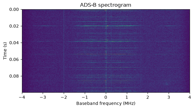
The following figure shows the spectrogram calculated with this approach for the beginning of an ADS-B recording that I have used as an example for the development of this receiver. With 10 ms of time span in the spectrogram, ADS-B messages are too brief to see well, but we can see the carriers of strong messages and get an idea of the typical frequency errors. The PSD plot shown above is the maximum of this spectrogram over the time axis.
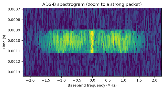
The following shows a zoom to a strong message. The centre of this message in the spectrogram corresponds to the best time alignment between the spectrogram grid and the message, and it is the local maximum that we want to detect.
A 2D detection of local maxima can be too expensive, and it is not really worth the effort. If two messages are transmitted at different frequencies and nearly at the same time, then it will be impossible to decode both of them, due to the collision. At most we will be able to decode one message if the other message is much weaker. Therefore, we can turn the local maxima detection problem into a 1D problem by taking the maximum over the frequency axis (limited to the central 4 MHz of the spectrogram). This shows how this maximum over frequency looks as a time series.
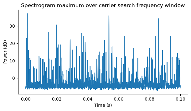
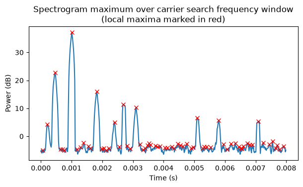
The first condition I impose to consider a point in this time series as a detection candidate is that it has to be a maximum in a window of ±2 time steps about it. The choice of the window length came as an educated guess based on the following considerations. The duration of a Mode-S long reply in the spectrogram is a window of ±7 time steps. However, we want to attempt to decode messages that overlap partially in time, so we want to have a narrower window for this condition. The window cannot be too small either, since that would cause too many time steps in random noise to pass the check, and it could also cause messages to be detected multiple times, which could lead to duplicated decodes that we need de-duplicate. A window of ±2 time steps gives a sweet spot. With 5 steps in total, the probability that random noise passes the check is 1/5, and it is very unlikely to get multiple detections for the same message. If there are multiple detections of the same message, they must be at least 3 time steps apart, which given how the search for the message alignment is done (see below), implies that at most one of these detections will be a correct decode, thus eliminating any chance of duplicated decodes.
The following plot shows the beginning of the time domain plot with the local maxima detected with this test marked in red. We can see that each message is detected once, and there are many spurious detections in the noise floor.
We need to add an additional condition that removes most of the noise floor local maxima. A possible approach is to estimate the noise floor power and then require the maxima to be some constant above the noise floor level. However, as I have argued above, it is difficult to estimate the noise floor in a scenario where there are many messages per second.
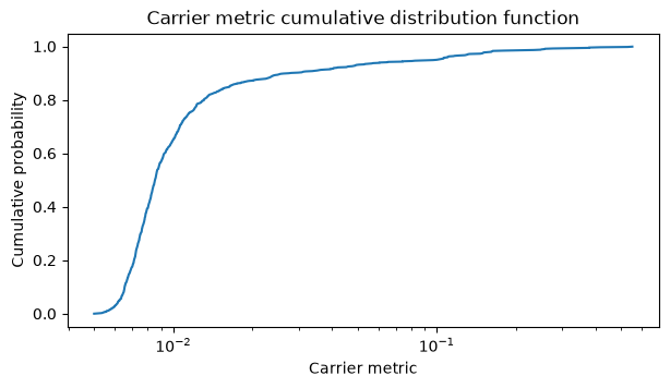
A look at the PSD of the signal suggests an alternative idea: using the SNR of the residual carrier in the spectrogram. The data power counts as noise in this SNR calculation, so for high enough CN0 this SNR measurement is dominated by the data modulation and tends to a constant as the CN0 increases. For low CN0 the SNR measurement is dominated by the noise floor, since the data modulation is below the noise. Even though this SNR saturates for high CN0, it gives a good way of setting the detection threshold. I use what I call the carrier metric, which is the quotient between the power of the spectrogram point corresponding to the carrier (the local maximum that is a candidate) and the integrated power in the rest of the spectrogram (only the central 4 MHz), minus a notch of ±200 kHz around the carrier frequency bin. The notch makes this quotient a carrier versus data plus noise comparison, and it also excludes the carriers of most messages that might overlap partially in time with this message.
The following plot shows the cumulative distribution function of this carrier metric in my test recording. A reasonable choice for the carrier metric threshold is 0.015, which is in the knee of this curve. This choice can be refined further by doing false detection simulation more systematically (which is what I show later).
The following figure shows the detections obtained with this carrier metric threshold. This has eliminated all the candidates in the noise floor.
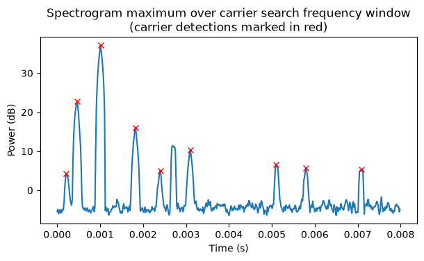
We can also see an RF burst at around 2.8 ms that has not been detected. Looking at the corresponding part of the waterfall in Inspectrum we see that this burst is a Mode-A/C reply. The Mode-A/C modulation does not have 50% of the message energy concentrated in a residual carrier, so this carrier metric has the added advantage of filtering out some Mode-A/C replies, especially if they have high SNR (there is a lower SNR Mode-A/C reply at 7.1 ms that gets detected).
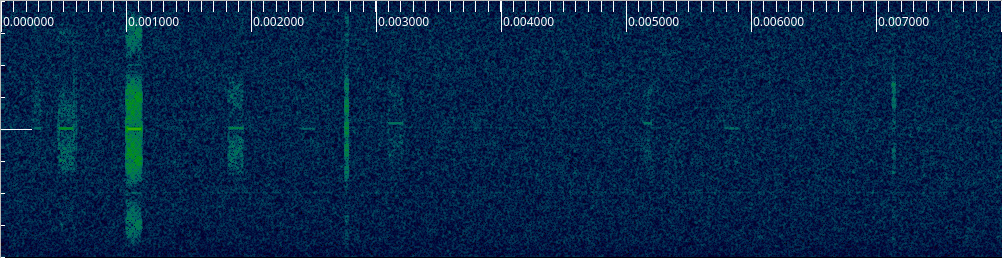
Also note that this carrier detection algorithm is detecting quite clearly some ADS-B messages that are very faint on the Inspectrum waterfall. This shows the advantage of using a message detection method that integrates 50% of the message energy.
Message demodulation and decoding
After obtaining a message detection with the method outlined above, we can obtain a fine carrier frequency estimate by taking the FFT bin corresponding to the detection and its two neighbouring bins and performing parabolic interpolation to obtain sub-bin resolution. This gives a rather accurate estimate, often well below 0.1 times the inverse of the duration of the message.
On the other hand, we only have a coarse time estimate for the message. In high SNR, the time step where the maximum detection happens will be the closest one to the true message time, so at most we can be wrong by 64 samples. However, in lower SNR, noise can make the maximum appear at one of the adjacent time steps, and then we get a time error that is larger than 64 samples. Additionally, the contribution of the 4 pulses in the Mode-S preamble causes a bias that tends to favour negative time errors (the message payload is detected before its true location). To be conservative and robust we should assume that the message time estimate can be wrong by up to ±128 samples.
With this in mind, given a detection, we extract the IQ samples at the location corresponding to the detection, plus 128 extra samples on either end, plus a few (3) extra samples on the right end to make the remaining operations simple. The following shows the IQ samples in this window for the example strong packet that was shown above.
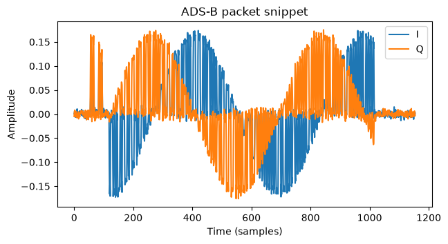
It is apparent in this plot that there is a carrier frequency error. Since we have estimated that from the carrier detection, we can remove it. After removing it, we can estimate the carrier phase by averaging the samples in the nominal window corresponding to the Mode-S payload (that is, 896 samples assuming that the detection has zero time error). We can also remove this estimated carrier phase, obtaining the samples shown below, where most of the message power is in the real and positive component.
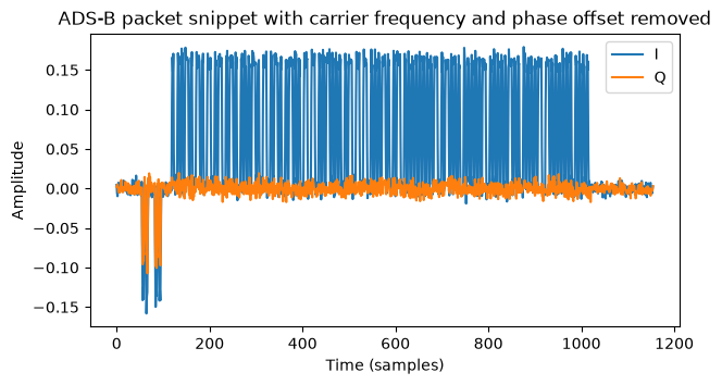
Interestingly we see that the preamble pulses are transmitted with a different carrier phase. I don’t know how common this is, but in any case we will not be using the preamble at all.
As I motivated above, our strategy for symbol and message time alignment is a brute force search using blind decoding. We are at 4 samples per pulse, and we only consider clock phases which are an integer amount of samples. Therefore, there are four possible clock phases. For each of these, we integrate pulses with a rectangular pulse shape filter (that is, we take groups of 4 samples and add them). The results are shown here. In this case the third clock phase is the one that gives the best results.
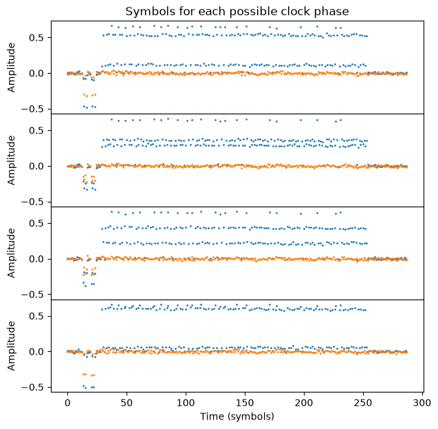
Due to the PPM modulation there are two possible cases for pairing these pulses as the two location candidates for each bit. We can either pair (0,1), (2,3), …, or (1,2), (3,4), … For each of the four clock phases, and for each of the two possible pairings, we perform coherent demodulation by choosing a 1 or a 0 for each pair according to which of the two pulse locations in the pair has larger (more positive) real part. This gives us 8 different sequences of hard bits. Additionally, we also perform noncoherent demodulation in a similar way, but comparing the complex magnitude of the two pulse locations in each pair. Noncoherent demodulation does not add much CPU usage, and although it is less sensitive than coherent demodulation, it gives us a fallback for the case when carrier frequency and phase estimation fails (for instance because the estimate is disturbed by interference from another message).
Therefore, we have a total of 16 sequences of hard bits. One of them is supposed to contain the ADS-B message at some offset. We perform blind decoding by testing the CRC-24 in all these sequences and at all possible offsets until we obtain a successful CRC check. This approach has a major drawback. The CRC-24 that is used in Mode-S messages unfortunately initializes its register to zero and does not perform a final XOR. This is problematic when trying to find the correct message alignment with a CRC check. For instance, if the last bit of the CRC is zero and the bit preceding the message in the demodulation output is also zero, then we also get a successful CRC check for the message candidate that starts one bit too early. More generally, a circular shift of a message with correct CRC also has correct CRC as long as the bits that are being shifted from the beginning to the end or vice versa are all zeros (if some of these bits are ones, then this property is not true in general).
In order to increase the receiver sensitivity, it is common to correct up to 2 bit errors in ADS-B receivers. This error correction also interacts with the CRC circular shift property to increase the number of correct CRC checks at wrong locations. For instance, if the last bit of the CRC is zero and the bit preceding the message is one, the candidate that starts one bit too early has a correct CRC if its first bit is flipped to correct one bit error. Additionally, because we test on the order of 256 bit offsets for the message, and using up to 2 bit flips each offset contributes 6329 different messages, the CRC check is applied to a total of 1620224 messages (which are all different in general). This is 9.7% of \(2^{24}\), so false correct CRC checks because of random luck are not so uncommon.
The more1090 receiver has several mechanisms to cut down the number of false correct CRC checks. The first is testing the contents of some message fields (after applying the bit error corrections). The DF field (5 bits) must be 17 or 18, since these are the only values used for extended squitter. For DF17 messages, the CA field (3 bits) must be valid (0, 4, 5, 6, or 7, since the remaining values are reserved), and for DF18 messages, the CF field (3 bits) must be valid (0, 2, 3, 4, 5, or 6). The DF field test essentially catches all the candidates that are at a small time offset from the correct candidate and that happen to give a correct CRC check (modulo up to 2 bit errors) because of the circular shift properties of the CRC.
Another mechanism is to use a CN0 estimate, which I will describe below, to remove candidates with 2 bit errors that give a CN0 estimate below a certain threshold (67 dB·Hz by default). Noncoherent demodulation is also a source of false decodes. In random noise or interference, the noncoherent demodulation bits and the coherent demodulation bits are independent, so the noncoherent demodulation is another die roll at getting a correct CRC check with a random input. The strategy we follow to reduce this effect is to establish a certain threshold for the Hamming distance between the coherent and noncoherent demodulations of the message candidate (8 bits by default). When there are two bit errors in noncoherent demodulation and the Hamming distance is greater than or equal to this threshold, we use a higher CN0 threshold (71 dB·Hz by default).
With all these mechanisms in place, the false decode probability is cut down to around 0.35%. However, this still gives frequent false decodes. For instance, in a scenario with 1000 messages per second, we will see about 3.5 false decodes per second. It is difficult to reduce the number of false decodes further without reducing the receiver sensitivity significantly. In many use cases these false decodes can easily be filtered out because they give nonsensical data or because they correspond to an ICAO address that has only been seen once.
Decode candidates are ranked according to the following criteria in order of precedence: number of corrected bit errors (preferring candidates with fewer bit errors), demodulation type (preferring coherent demodulation candidates) and CN0 estimate. The best candidate according to these criteria is chosen as the message decode.
The CN0 estimator works as follows. Since the message bits are known, the signal plus noise power can be computed by adding the power in the pulse locations that correspond to the message bits (this uses the coherently integrated pulses shown in the plot above). To estimate noise power, we could follow a similar approach, adding the power of the pulse locations where the message says that there should be no pulse. However the problem with this approach is that when the message is not well aligned to an integer sample, the message pulses leak power into the adjacent noise pulses. Therefore, instead of taking the 4 samples in the noise pulse, we only take the central 2 samples, to avoid the potential leakage into the samples on the edges. This has the drawback that we get a wider filter shape for the noise measurement, so the impact from adjacent channel interference such as DME/TACAN on the noise estimate is larger than the impact on the Mode-S waveform. However, there is no easy way of improving this.
After the message is decoded, a time of arrival estimate with subsample resolution is computed. This is done based on the sample alignment corresponding to the best decode candidate. However, in some cases this candidate alignment differs by one sample from the optimal alignment. The reason is that in cases of low CN0 or interference, the optimal alignment might not decode correctly and therefore not be considered as a candidate. To solve this, the message powers for the candidate alignment and the alignments corresponding to one sample earlier and one sample later are compared, and the one that gives the maximum power is chosen as the best integer sample time for the message. Then the message power of alignments one sample earlier and one sample later than this are computed. Parabolic interpolation with these three points is used to obtain subsample resolution.
Simulator
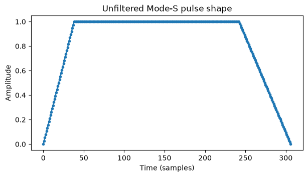
The more1090 simulator can generate all Mode-S and Mode-A/C reply message types. A polyphase filterbank is used to generate the pulse shapes in a way that can accurately represent arbitrary fractional message delays. For Mode-S, the prototype filter is designed at 64 times the sample rate (512 Msps). The filter is designed by starting with an unfiltered pulse shape that is a trapezoidal pulse with rise and fall times given by the typical values in the specification.
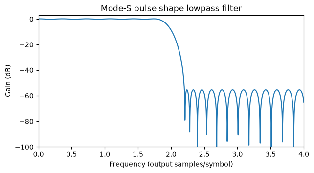
A lowpass filter with a cutoff at 4 MHz is designed using pm-remez. This filter models the effects of receiving the waveform with a receiver with only 8 MHz of bandwidth.
The convolution between the unfiltered pulse and the lowpass filter gives a filtered pulse that is used as the prototype filter. This is shown here in the time and frequency domains.
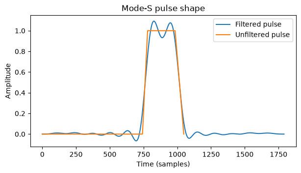
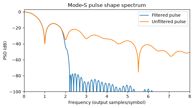
The polyphase filterbank runs as an interpolator that upsamples by a nominal rate of 4 the sequence of message pulses. The interpolator accepts a clock rate error that models a sampling frequency offset in the transmitter or receiver.
The Mode-A/C pulses are also generated with a polyphase filterbank, but the design of this is trickier. The Mode-A/C waveform has pulses with a nominal duration of 0.45 usec and gaps of 1 usec between pulses. The approach I have taken to generate these pulses is to divide the 1.45 usec interval into three parts. A pulse and its gap are represented by a one and two zeros at the input of the polyphase filterbank resampler. The resampler runs at a nominal rate of 1450/1500 x 4, and the prototype filter corresponds to a 0.45 usec pulse at this nominal rate (1500/1450 x 512 Msps). The construction of the prototype is analogous: we take a trapezoidal unfiltered pulse with rise and fall times given by typical values in the spec, we design a lowpass filter with a cutoff of 4 MHz, and we generate the prototype as the convolution of these two sequences.
The simulator generates messages according to the following parameters: message contents, timestamp (time of arrival), CN0, carrier frequency offset, carrier phase, and symbol clock frequency error. For the carrier frequency offset, carrier phase and symbol clock frequency error, random distributions are used by default. The carrier frequency offset is modelled as a normal with a standard deviation of 100 kHz, clamped to ±1 MHz. The carrier phase is uniformly distributed. The symbol clock error is uniformly distributed in ±50 ppm.
For the CN0, some simulations are done at a fixed CN0. Other simulations use a CN0 distribution that comes from a simplified model that takes into account distance to the transmitter and free space path loss. This models the transmitters as being uniformly distributed on a disk such that the receiver is on the axis through the centre of the disk, at a certain distance to the disk centre, and so that the disk radius is adjusted to give a certain distance between the receiver and the disk edge. Together with a maximum CN0 (corresponding to a transmitter at the centre of the disk) and free space path loss, this gives a CN0 model. This simplified disk model is applicable both to a terrestrial receiver scenario, where the disk models airplanes at cruise altitude, some 10 km above the receiver, and up to a maximum distance on the order of 500 km, and also to a LEO satellite receiver scenario, where the disk also models airplanes at cruise altitude, which are now some 500 km below the receiver, and up to a maximum distance on the order of 2600 km.
The simulator supports generating the following message types. Each message type has a corresponding generator function that produces random well-formed messages.
- Mode-S extended squitter messages (DF17 and DF18).
- Mode-S acquisition squitter messages (DF11 with plain CRC-24).
- Mode-S short messages using address parity (DF0, DF4, DF5).
- Mode-S all-call reply messages using parity/interrogator identifier (DF11 with interrogator identifier overlaid on the CRC-24 field).
- Mode-S long messages using address parity (DF16, DF20, DF21, DF24-31).
- Mode-S military extended squitter messages (DF19).
- Mode-A/C reply messages.
There are two ways of using the simulator. It can be used to generate a single message, where the output is a snippet of IQ samples that contains a given message with some fixed time, CN0, etc. parameters (which can be drawn from random distributions). It can also be used to generate a scenario, which contains many messages spread over a certain duration. In the scenario, each message type is generated as an independent Poisson process, which indicates the times of arrival of the messages according to an average number of messages per second. The way that this is actually implemented is as a single Poisson process, corresponding to all the message types, and then for each message its type is drawn randomly according to their relative probabilities. Reasonable defaults are given for these relative probabilities based on real world studies of the relative frequencies of SSR reply message types.
Benchmark results
The two modes of the simulator are used to benchmark the more1090 ADS-B receiver. The single-message mode allows us to test what happens at fixed CN0 over AWGN with individual messages that do not collide. The scenario mode allows benchmarking the behaviour in realistic situations with colliding messages and different CN0s.
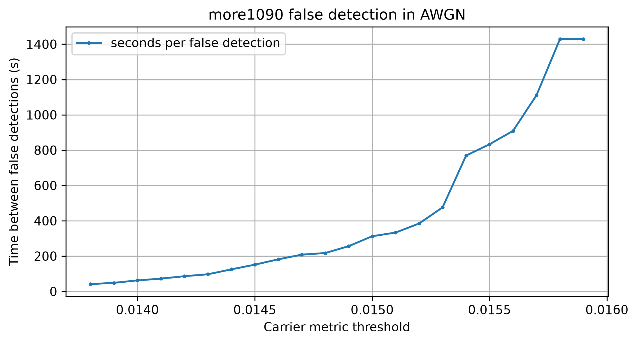
First a sweep in the carrier metric threshold running the receiver over AWGN is used to choose a default threshold that sets the operating point according to the desired mean time between false detections. The chosen default is 0.0148, which gives around 217 seconds between false detections. Tuning this setting is not too critical for real world operation in most cases. Unless the antenna is disconnected, the receiver is going to see Mode-S messages (perhaps quite weak), which will trigger the carrier detection, and will sometimes result in false decodes, with a typical rate much higher than one decode every 200 seconds.
In many of the following plots the CN0 of the message is used for the horizontal axis. Because the Mode-S modulation has 50% duty cycle, there are several possible definitions of CN0 that can make sense to use. Here the definition I’m using is the one that takes into account the pulse power (or the message peak power). A definition that takes into account the message average power instead gives a CN0 that is 3 dB lower, because the average power is 50% of the peak power.
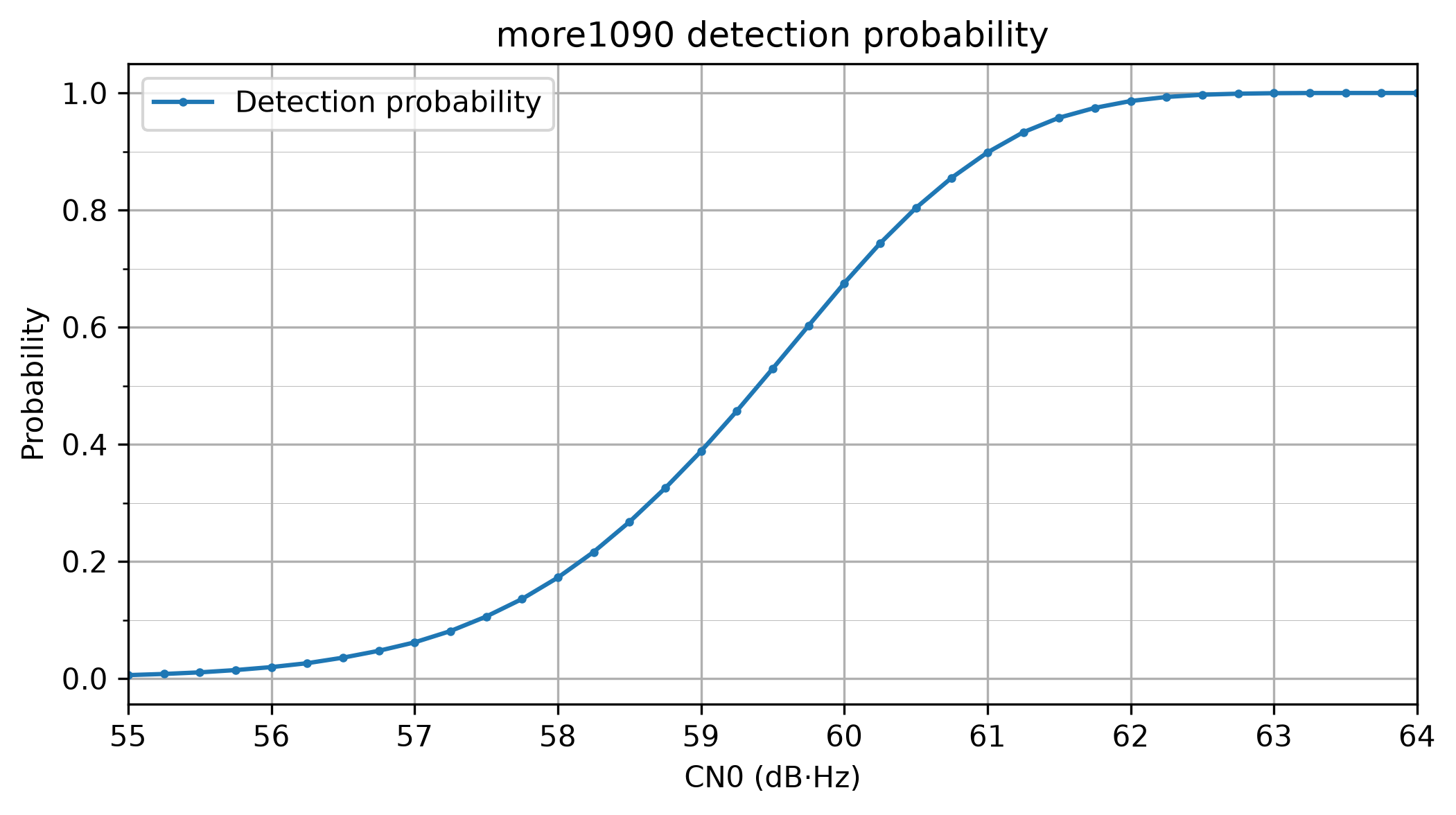
Once the carrier detection threshold is defined, we can test the detection probability of single ADS-B messages in AWGN. We see that the detection threshold is around 59.5 dB·Hz, where 50% of the messages are detected.
The following plot of decoding probability is somewhat difficult to read, but it is very informational, as it aggregates a lot of data. First, dashed lines show the theoretical decode probability for coherent demodulation. This relates coherent PPM demodulation with coherent demodulation of Manchester coded BPSK, so these curves follow from the well-known BER vs Eb/N0 curve for coherent BPSK. The different curves show the successful decode probabilities correcting up to 2, 1 and 0 bit errors, and also the probabilities that the number of bit errors was exactly 1 and exactly 2. Dotted lines show the same for noncoherent demodulation. Because the PPM pulse positions are orthogonal, these curves follow from the well-known BER vs Eb/N0 curve for noncoherent FSK with orthogonal symbols. The actual performance of the more1090 receiver in simulation is shown with solid lines.
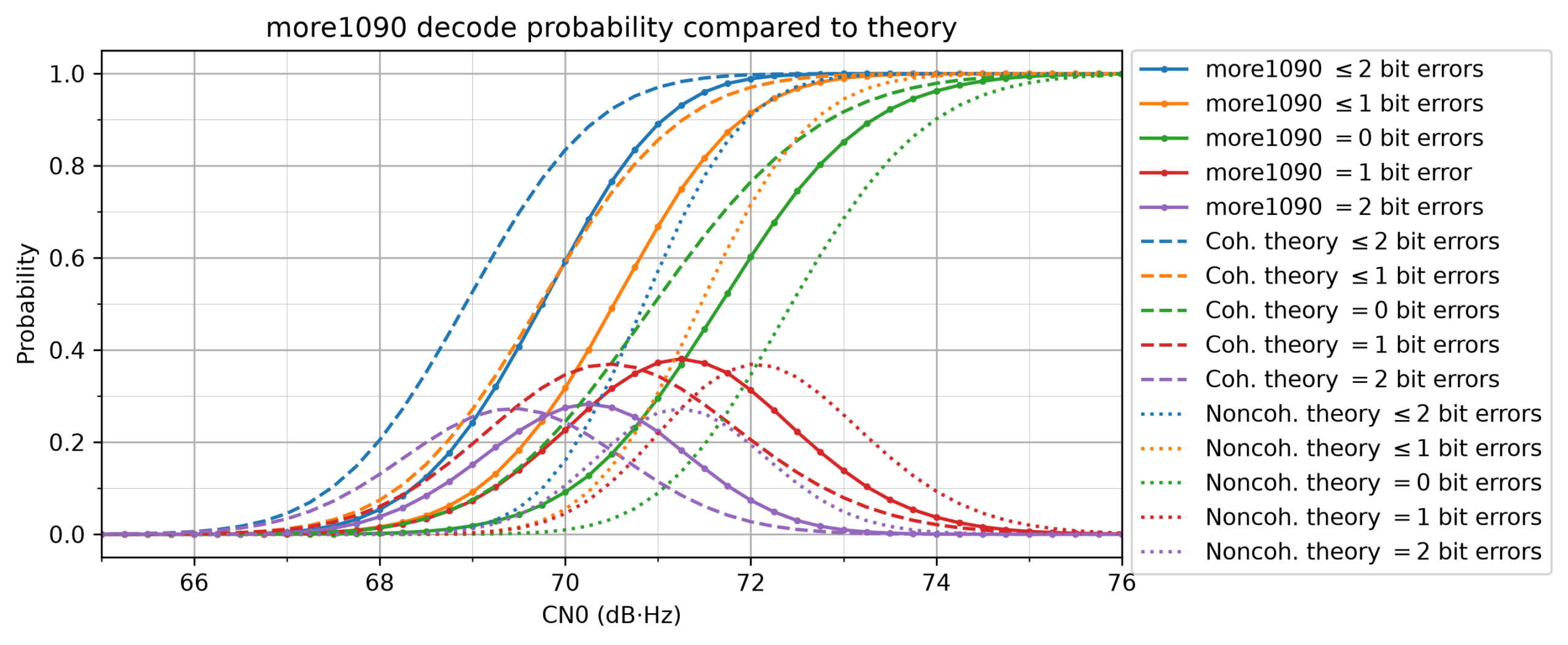
We see that more1090 is performing roughly 0.8 dB worse than coherent demodulation theory. This is great, because having less than 1 dB of implementation losses in a full modem chain is usually quite good, unless the modem has been designed very carefully to minimize the losses (such as in very sensitive modems for deep space communications). Here I believe that the main contributor to implementation losses is the fact that we are using 4 samples per symbol and only testing clock offsets that are an integer number of samples (as I mentioned above, this gives a worst case loss of 1.8 dB).
We can also see that in theory coherent demodulation is almost 2 dB better than noncoherent demodulation. This is a strong reason for implementing coherent demodulation. Finally, note that the theory predicts that decoding below 66 dB·Hz is basically impossible, whereas more1090 can detect almost all messages above 63 dB·Hz. This means that the FFT-based carrier detection algorithm is more than sensitive enough for our needs.
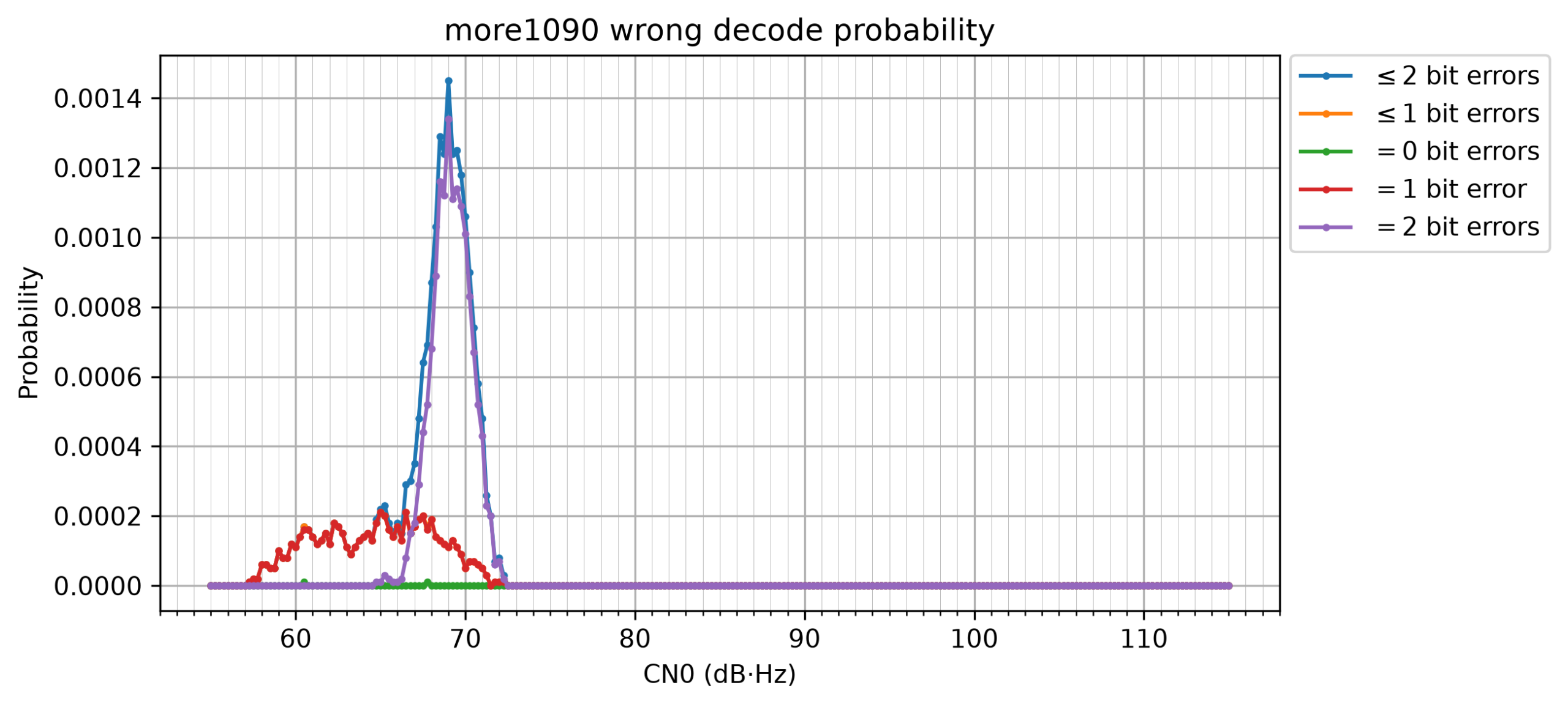
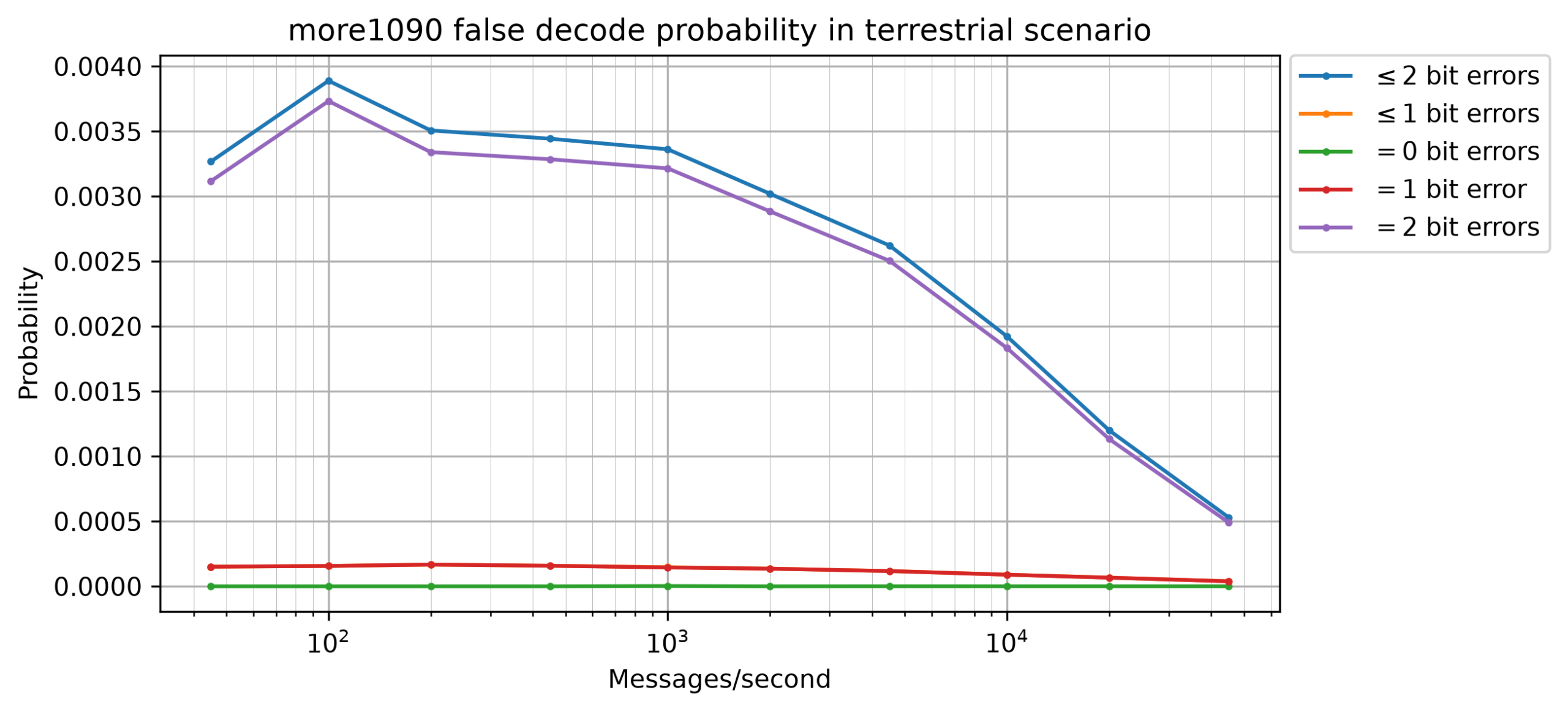
The following figure shows the wrong decode probability. This is the probability that when seeing an ADS-B message, the receiver produced a message that passed all the checks but does not match the original message. We can see that allowing 2 bit error correction produces a relatively large amount of wrong decodes, which is highly reduced by the additional CN0 checks that we have established, but it is still noticeable. A wrong decode probability of 0.1% might seem low, but in ADS-B there are real world scenarios that have 1000 messages per second or more.
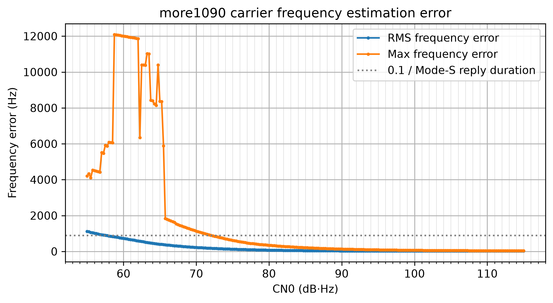
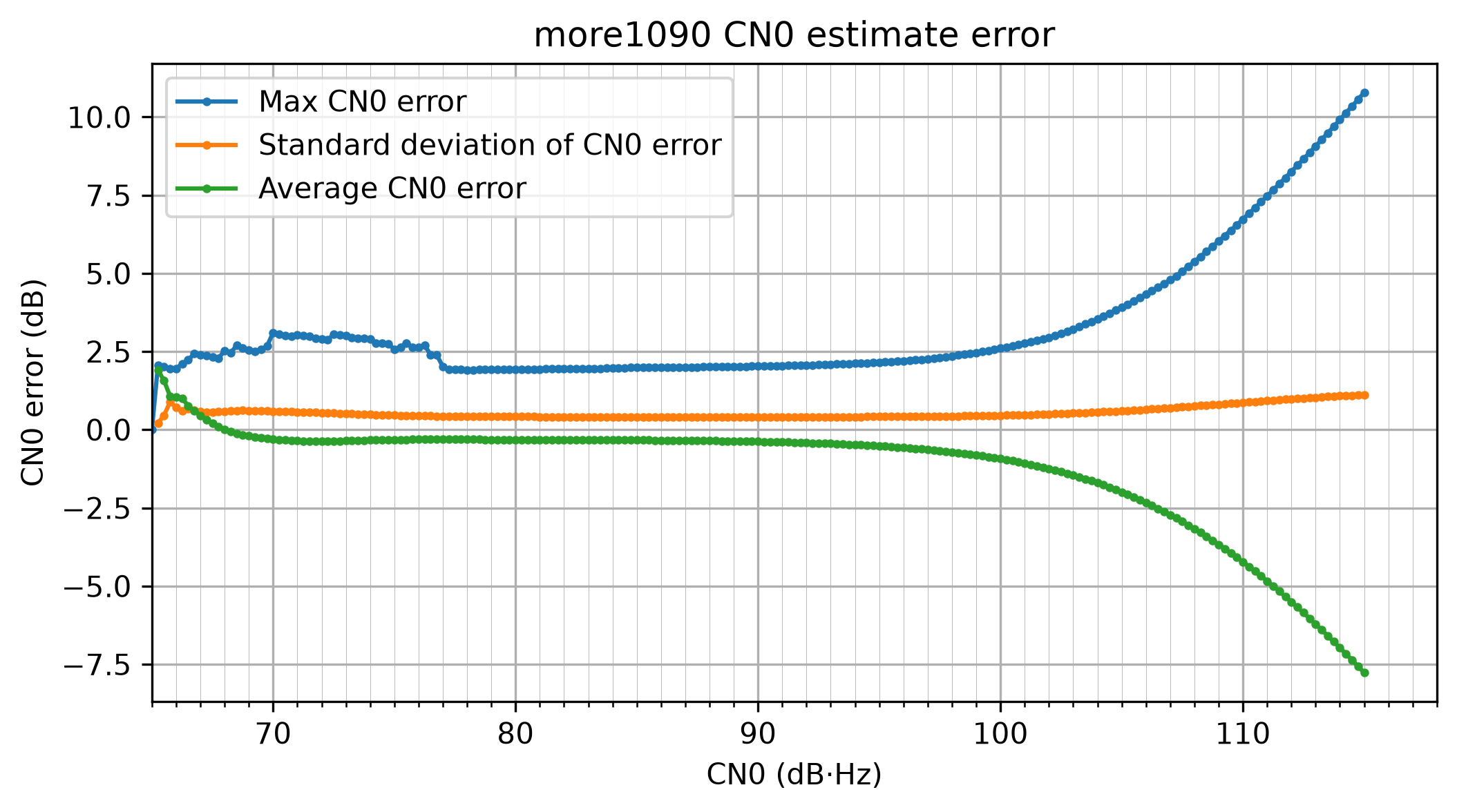
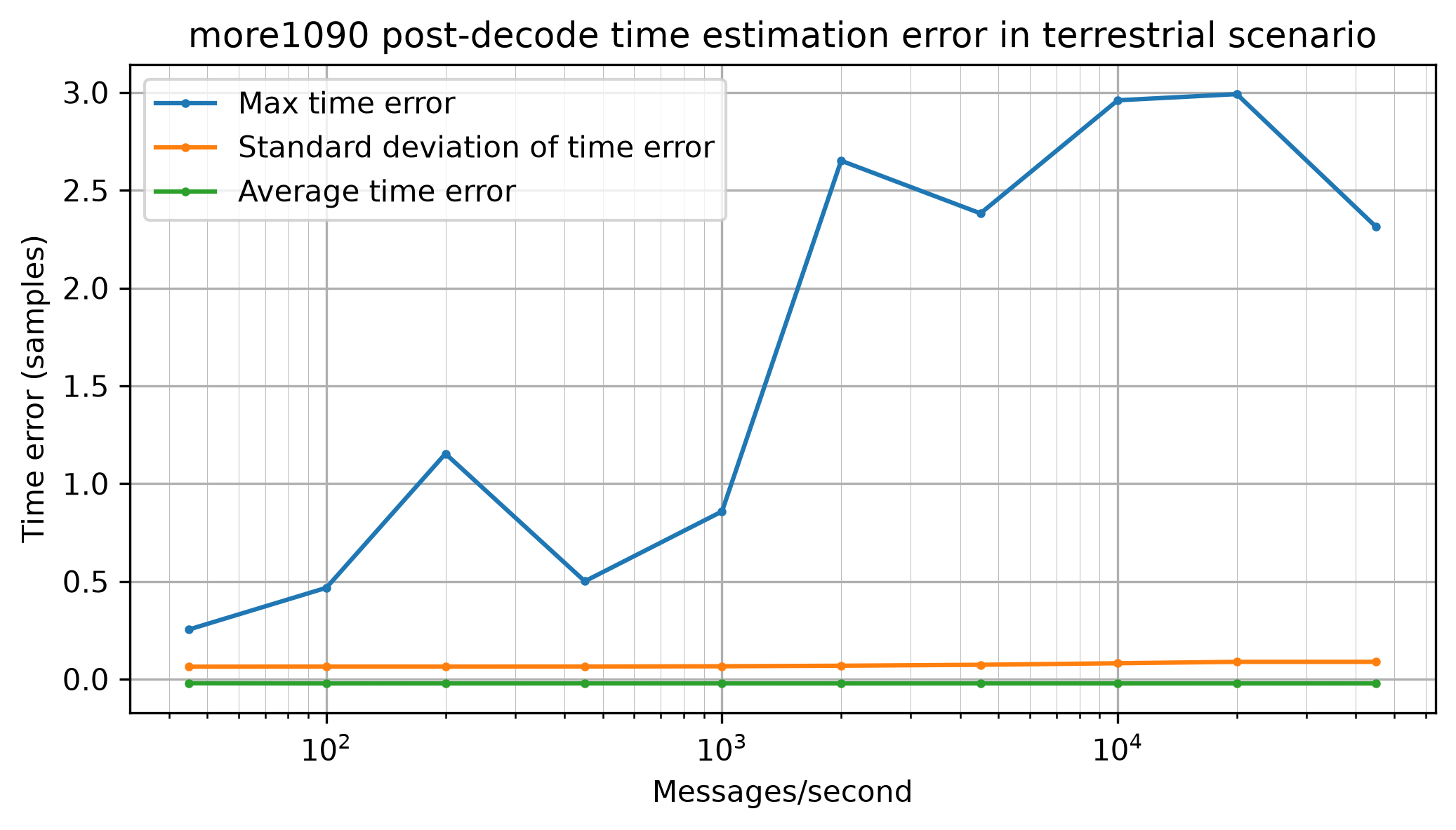
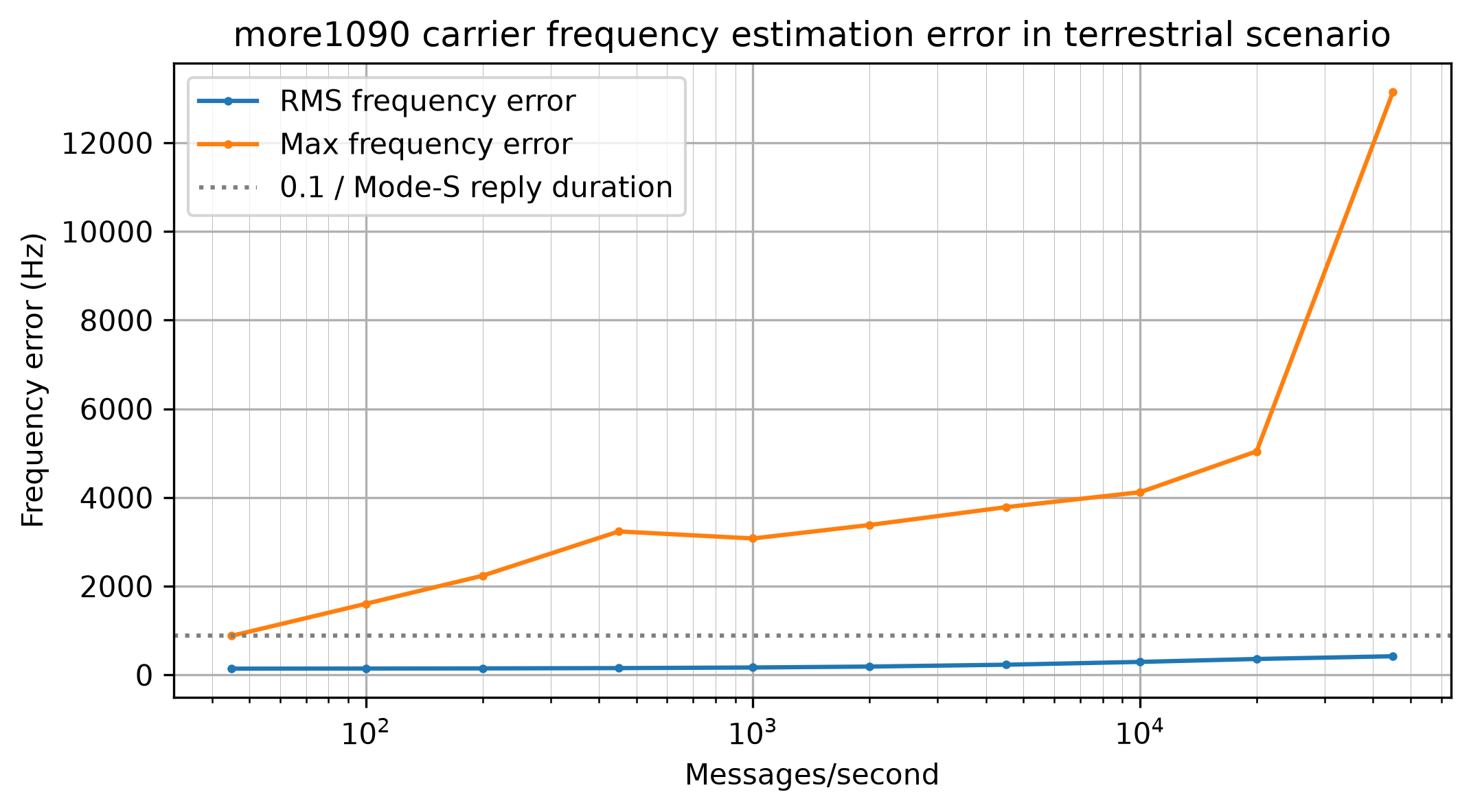
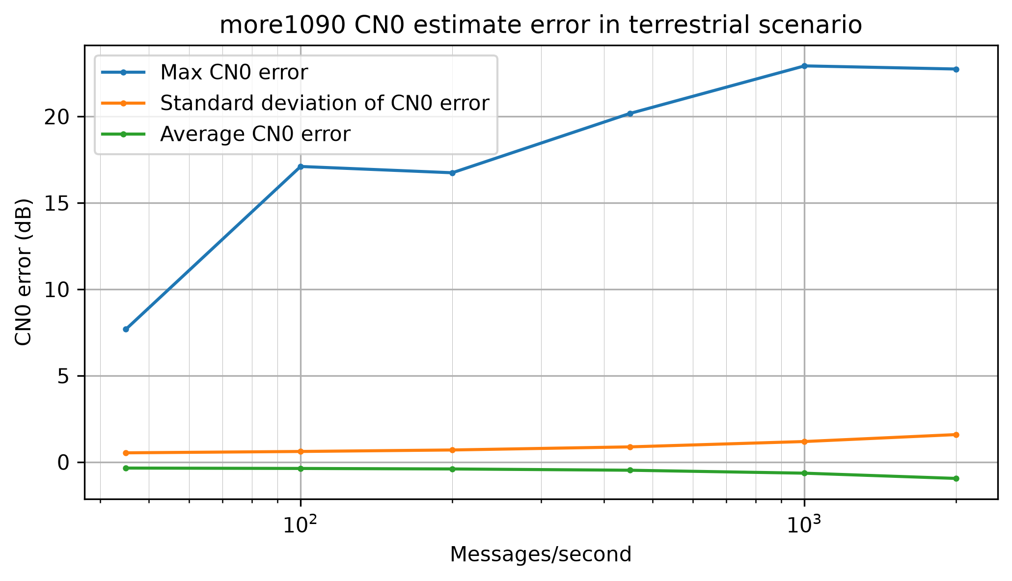
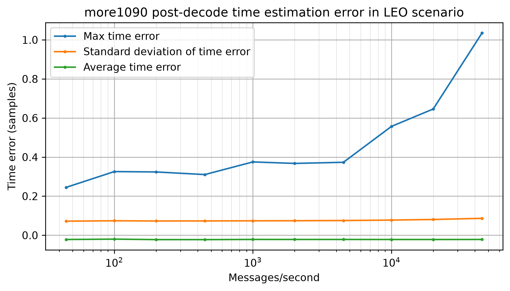
The more1090 receiver produces time, frequency and CN0 estimates for decoded messages. The following plots evaluate the error of these estimates, taking into account only messages that are successfully decoded (and excluding wrong decodes).
To evaluate the time error we need to take into account the fact that the more1090 simulator is using a polyphase filterbank to modulate the Mode-S messages, while the receiver is using a rectangular pulse shape. The mismatch between the pulse shapes causes an estimator bias that depends on the fractional sample delay of the message. While for a fixed fractional sample delay the average time error converges to this bias and the standard deviation of the time error converges to zero as the CN0 grows, the plot below considers a uniformly distributed fractional sample delay. This is the reason why the standard deviation does not converge to zero.
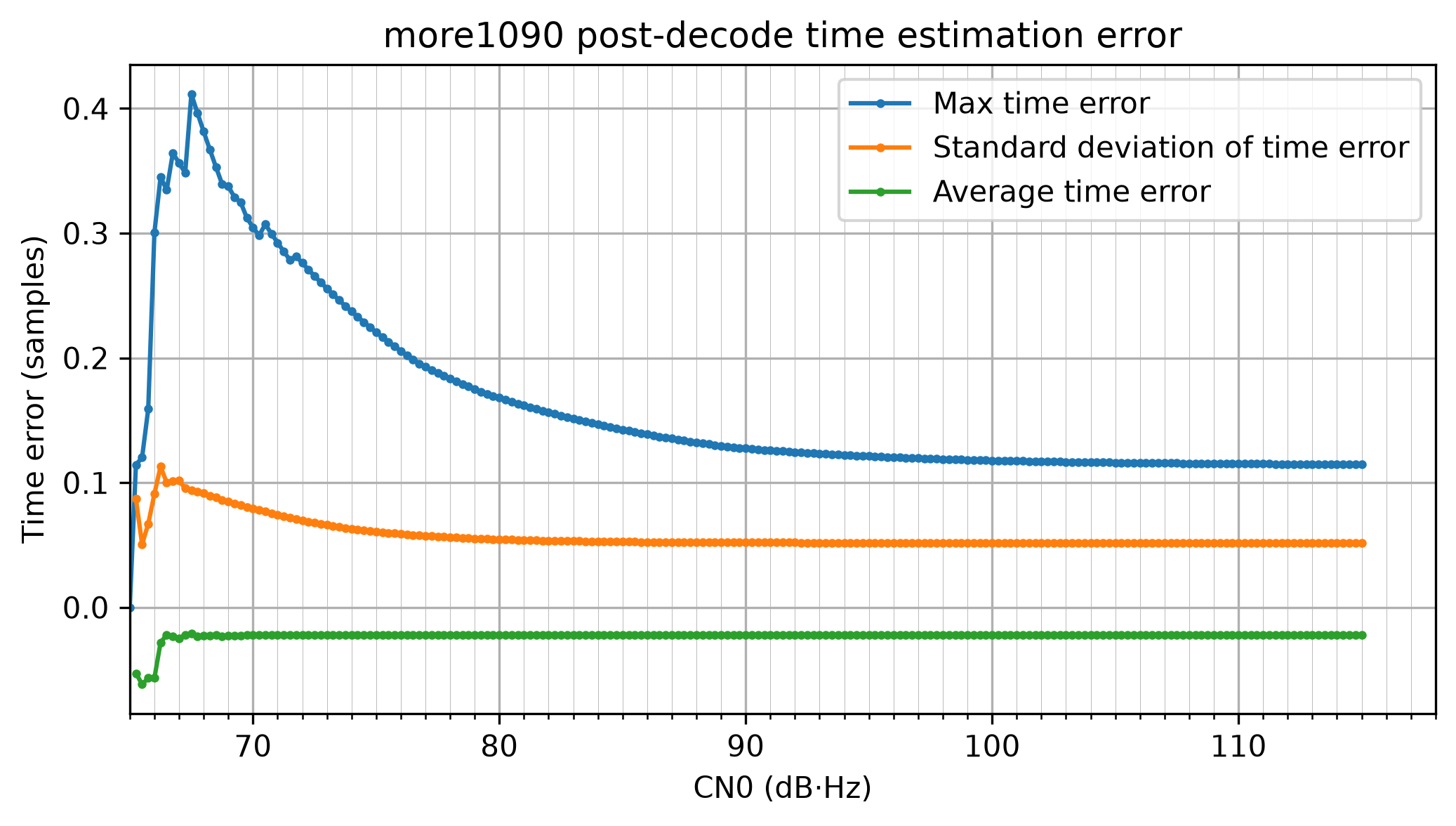
What happens with the particular pulse shape used by the simulator is not very relevant. In the real world the pulse shape depends on the transmitter and also on the receiver filtering. Therefore, it does not make sense to optimize the receiver or the estimator to any particular pulse shape. However these simulation results give us an idea of what to expect in real world cases. The typical time error will be around 0.06 samples, which is around 7.5 ns, or 2.25 meters.
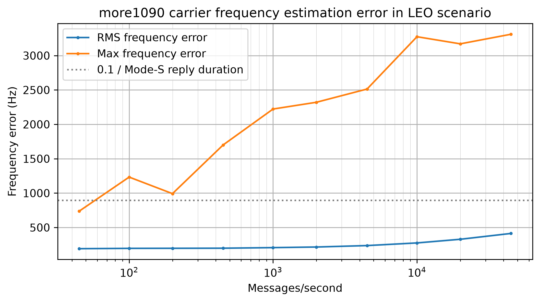
The following plot shows the frequency estimation error. This plot considers all detected messages, not only successfully decoded messages. At low CN0 the maximum error is pretty high. This means that there are some cases for which the peak FFT bin is several bins away from the correct location (the bin width is 2.2 kHz). However the RMS frequency error does not show a large error, which means that these messages with a large error are relatively few. A dotted line marks 0.1 divided by the Mode-S long payload duration (112 usec), which is 893 Hz. This corresponds to a rule of thumb for when the frequency error causes negligible losses in coherent demodulation (this frequency error causes a rotation of 0.1 cycles over the whole message). We see that the frequency estimator is accurate enough for coherent demodulation above 66 dB·Hz, which is the range that we care about.
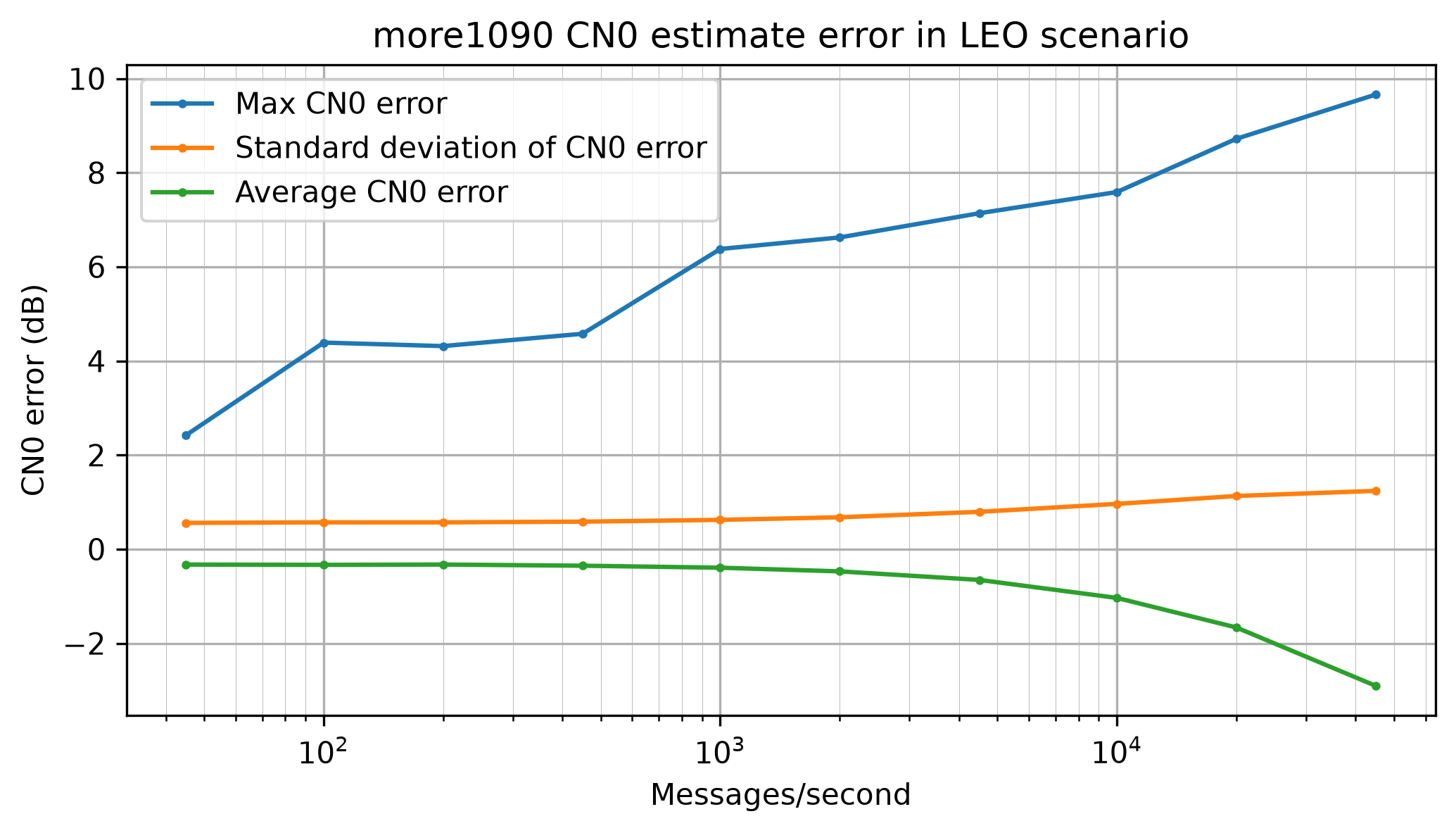
The following shows the CN0 estimate error for successfully decoded messages. We see that the estimate is pretty accurate for the main range of interest. However, the estimator underestimates significantly for very high CN0. For instance, at 115 dB·Hz, the estimator underestimates by about 7.5 dB·Hz. It is as if the estimator compresses when the CN0 gets too high. This is typical for many types of CN0 estimators. It is difficult to design a CN0 estimator that remains accurate at very high CN0, where signal distortions begin to matter. In this case, what happens is that the simulator pulse shape leaks some power in the samples that we are using to estimate the noise floor, and at very high CN0 that leakage power becomes larger than the noise power. Nevertheless, for many applications it is okay that the CN0 estimator saturates at very high CN0.
For benchmarking with the simulator in scenario mode, I have chosen two scenarios, which are representative of a terrestrial receiver and a LEO satellite receiver. For the terrestrial scenario I have considered a distance to the transmitters ranging between 10 km (cruise flight overhead) and 500 km (typically limited by line-of-sight range). I have taken educated guesses of 100 W EIRP for the transmitter, 4 dB noise figure for the receiver and an isotropic antenna. The free space path loss at 10 km is 113.2 dB, which would give 106.8 dB·Hz CN0. I have rounded this to a maximum CN0 of 105 dB·Hz.
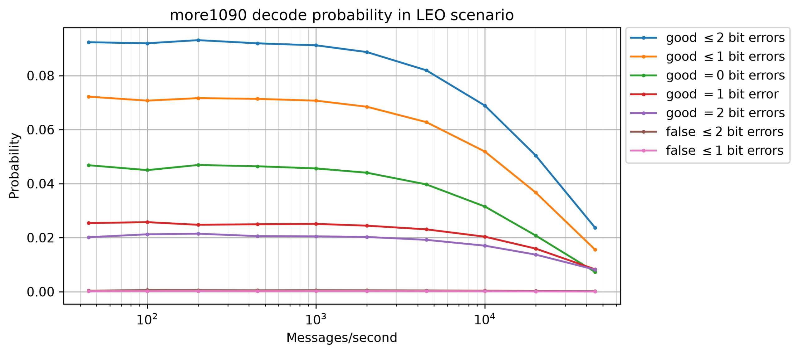
For the LEO satellite scenario I have considered a distance to the transmitters ranging between 500 km (flight directly below the satellite, with the satellite at an altitude of roughly 500 km) and 2600 km (slant range to the horizon at 500 km altitude). The free space path loss at 500 km is 147.2 dB, so with the same numbers as above this gives 72.8 dB·Hz. I have purposefully rounded this up to a maximum CN0 of 75 dB·Hz, which could account for more antenna gain at the satellite. The free space path loss at 2600 km is 14.3 dB larger than at 500 km, so in this scenario the simulator produces CN0s ranging between 60.7 dB·Hz and 75 dB·Hz. Due to the transmitter-on-a-disk model, lower CN0s are more frequent. Many messages are weaker than 66 dB·Hz and are impossible to decode, so they only serve to generate interference that makes decoding the stronger messages (which are the ones that stand a chance of being decoded) more difficult.
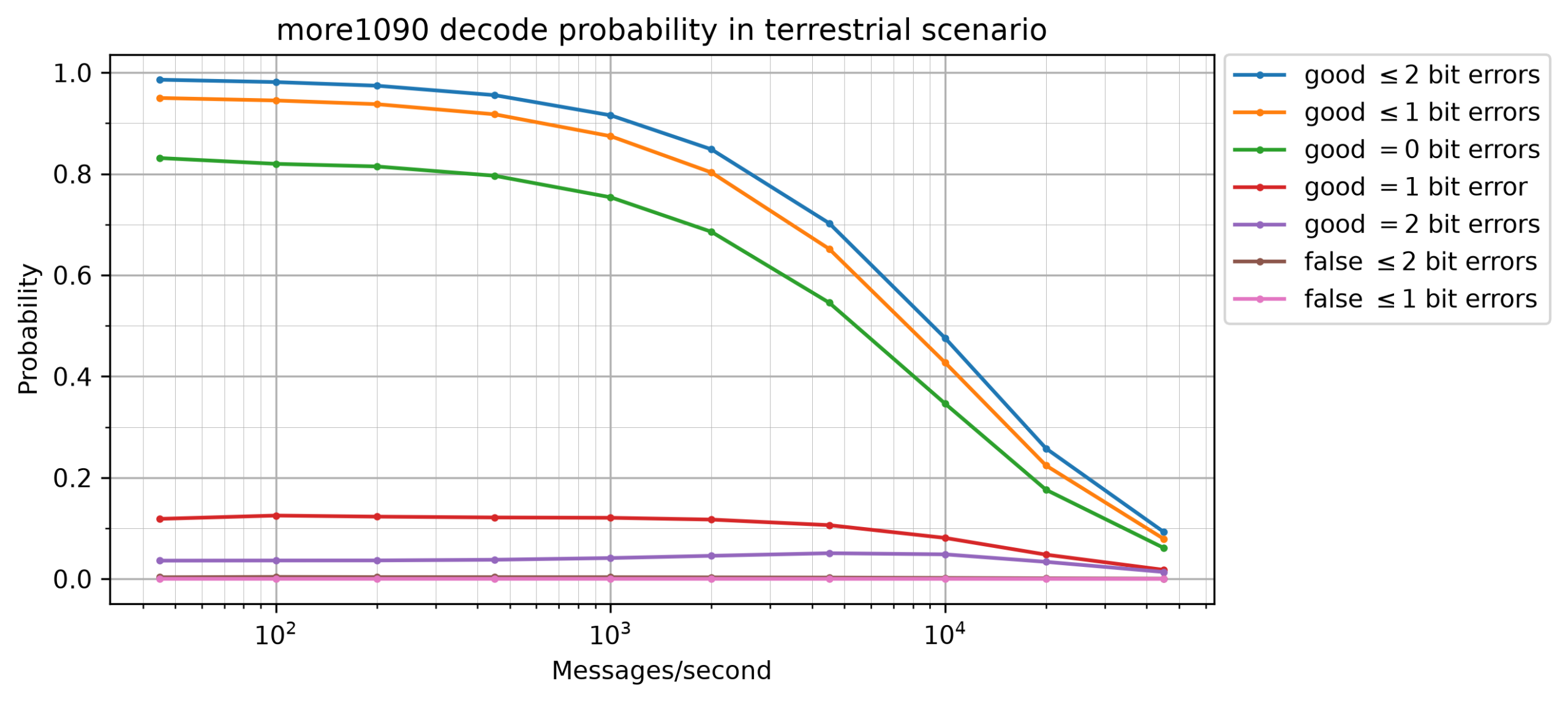
For each of the two scenario types, I have done multiple runs by varying the number of messages per second. This defines the total number of SSR reply messages that are simulated per second on average. Only 45% of these reply messages are extended squitter (ADS-B) messages. The following plot shows the ADS-B message collision probability depending on the number of messages per second. This is defined as the probability that another message (of any type) overlaps in time with an extended squitter message. The following plot shows the collision probability for the terrestrial scenario. The plot for the LEO scenario is identical, since the only difference between the two scenarios is the CN0 distribution.
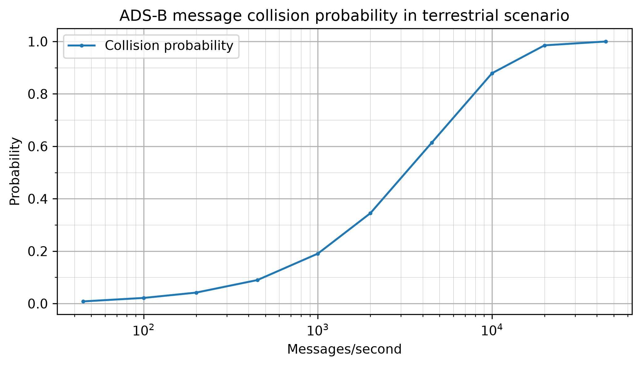
Real world terrestrial receiver busy scenarios have roughly 1000-2000 ADS-B messages per second, which here would correspond to 2222-4444 SSR messages per second. For a real world LEO scenario I don’t have a good estimate or model for the number of SSR messages per second. Note that this count should include all messages, including those from transmitters close to the horizon, which have a CN0 that is too low for decoding. Reasonable models would take into account geographic distribution and time of day. Perhaps a ballpark estimate can be obtained with ADS-B receiver network data. Regarding commercial receivers, the Satlab Polaris ADS-B receiver claims to be able to decode up to 8333 ADS-B messages per second. This number is basically the inverse of the ADS-B message duration of 120 usec, so I guess that this means that the receiver is able to process back-to-back ADS-B messages without dropping any (it has enough compute resources). I don’t think this specification of 8333 messages per second is based on a scenario where messages arrive at random times, since at that rate the collision probability is around 80% even if the traffic only consists of ADS-B messages (in the real world scenarios there are other message types in addition).
For completeness I have considered up to 45000 messages per second. This gives a collision probability of essentially 1 and gives a heavily degraded scenario in which the probability of successful decode falls off a cliff (although the number of correct decodes per second is still relatively high).
For the terrestrial scenario, we can see that at low numbers of messages per second more1090 can decode almost all messages. The decode probability is impacted as the number of messages per second keeps growing, and at 45000 messages per second only about 10% of the ADS-B messages can be decoded (but that is still around 2000 good ADS-B decodes per second, similar to the number of good ADS-B decodes per second for 10000 messages per second).
The next plot shows a detail of the false decode probability. This is defined as the number of messages decoded by more1090 that do not match any of the messages generated by the simulator, divided by the total number of extended squitter messages in the simulation. Here the probability is around 0.3%, which is worse than in the single-message tests. This is because in this scenario there are relatively strong messages that can contribute to false decodes by perturbing the CN0 estimate of overlapping false decodes, and causing them to pass the CN0 filters. Note that at 2000 messages per second there are 900 extended squitter messages per second, so the 0.3% false decode probability implies that we see around 2.7 false decodes per second.
In the LEO scenario we see that the decode probability is pretty low, around 9%, even for low numbers of messages per second. This is because the CN0 model generates many weaker packets that are just impossible to decode.
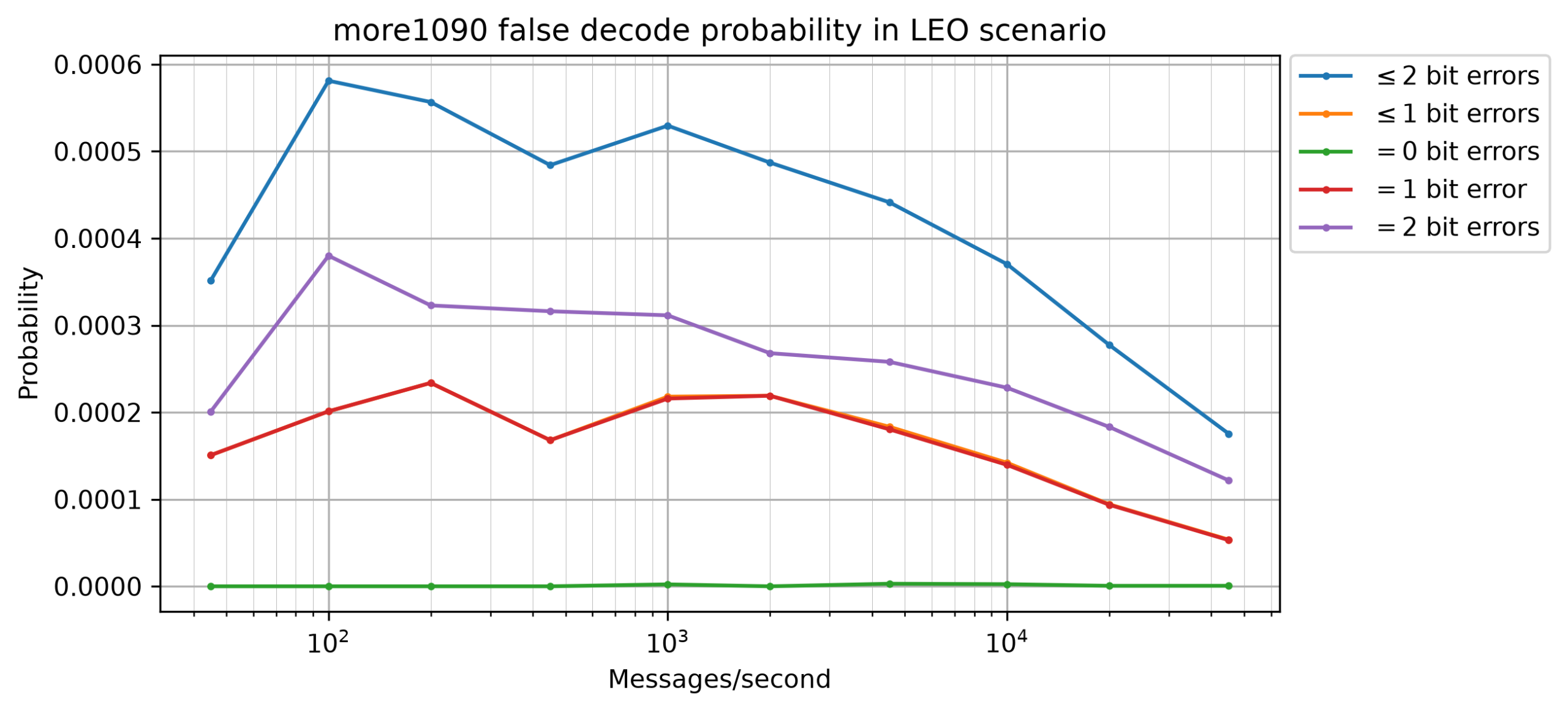
The false decode probability in this scenario is much lower, around 0.05%. This is in part because there are no strong messages, in contrast to the terrestrial scenario.
There are also plots for the errors of the time, frequency and CN0 estimators in each of these scenarios. The maximum errors are usually much larger than in the single-message tests, because in unlucky cases of collisions the estimate can have a large error. However, the average behaviour (standard deviation, mean and RMS) is similar to the single-message tests.
Here are the three plots for the terrestrial scenario.
And here are the three plots for the LEO scenario.
Comparison with readsb
Since this whole project began motivated by the poor sensitivity of existing open source ADS-B receivers such as readsb, I also wanted to do a simple comparison between more1090 and readsb. To me the fact that more1090 comes with performance curves that show that it is within less than 1 dB of the coherent demodulation theory and that it performs reasonably in busy scenarios, and that readsb does not have any kind of performance benchmarks, is already enough to highly prefer more1090. I don’t want to roast readsb by doing extensive benchmarks of its performance. However it is good to do some comparisons to understand how large the improvement is.
I made a 20 second IQ recording at 1090 MHz from my window (which has reasonably good line-of-sight visibility to the northern half of the sky) to serve me as an example for developing more1090. I used the same antenna as in my DME experiments, and a USRP B205mini. In this recording, more1090 decodes 2633 extended squitter messages, of which definitely 25 are false decodes according to some heuristics, because the message format is invalid in one way or another, and another 26 messages might be false decodes because they have 2 corrected bit errors and their ICAO address was only seen once. This leaves us with 2582 messages that are probably good.
readsb requires a 2.4 Msps input, so I have made a small GNU Radio flowgraph that decimates the 8 Msps 16-bit IQ recording to 2.4 Msps 16-bit IQ. I can run readsb on the resampled file as follows.
readsb --device-type ifile \
  --ifile ADS-B_8Msps_2026-08-27T08:36:39_readsb.ci16 \
  --iformat SC16 --raw
Since readsb decodes other types of messages besides extended squitter, for a fair comparison I filter the decodes to allow only extended squitter messages using a small Python script.
The whole pipeline is the following.
readsb --device-type ifile \
  --ifile ADS-B_8Msps_2026-08-27T08:36:39_readsb.ci16 \
  --iformat SC16 --raw | \
  ./filter_extended_squitter.py | wc -l
This gives 941 extended squitter messages, of which 2-7 messages might be false decodes according to the same criteria. Therefore, more1090 is decoding 2.75 times as many messages as readsb on this recording.
The results are more striking in a LEO scenario such as the one defined above. I generate such a scenario as follows.
more1090-simulator scenario \
  --min-distance 500 --max-distance 2600 --max-cn0 75 \
  --duration 20 --messages-per-second 10000 \
  leo-scenario.sigmf-data
Running more1090 on this scenario produces 6118 decoded messages, of which 35 are false decodes (here we can know exactly which messages are false decodes, because the simulator outputs ground truth as SigMF annotations). In contrast, readsb produces only 3 decoded extended squitter messages (all of which are good decodes).
AI usage
This project is the first open source project in which I have used AI significantly (professionally I have been using AI for a longer while). I’ll begin by saying that I know that there are strong feelings about AI in the open source community, including concerns about its negative impacts. As a mathematician I also cannot ignore the recent cases of extractive use of open problems in mathematical research. I share the concerns that have been expressed by the mathematical community. Nevertheless, at this point it is fully clear that AI is very useful to do technical work. The technology is evolving very rapidly, faster than what we can adapt to it and find good and reasonable ways to use it. Since this technology is not going to vanish, I think it is better to try to adapt to it and find a good path than refusing to use it altogether, even though I respect people who make that decision.
In this project my approach has been to use AI to write better software, not to write software faster. This point of view is inspired by the motivations of the Rust LLM policy. I have written all the code you can see in more1090 by hand. I have used AI mainly for the following tasks.
- Reviewing my code periodically, after making a batch of changes. This has been very useful because the AI spotted problems much earlier than I would normally. I should also say that AI code reviews can still have blind spots. For quite a long while I had a bug in the function that checks carrier detection. I had made a silly mistake and I was checking if the candidate is a local maximum in a ±2 element window about it in the frequency dimension, rather than in the time dimension. Because the candidate is chosen as the maximum FFT bin, this check was trivially satisfied all the time (the carrier metric threshold check was the only thing limiting candidates). AI never noticed this mistake, and I only noticed this while re-reading and slightly refactoring the code to add more unit tests.
- Examining where test coverage is lacking and proposing ideas for unit tests. I have always thought that test coverage reports have very limited usefulness. They just say whether a line of code has been executed by tests or not, but they do not say anything about whether meaningful checks have been done about the functionality of that line. AI can do this, and even if what it says is not 100% accurate, it is still useful. Occasionally I have even used AI to generate code for new unit tests, but I’ve only used this as an example to see what checks could be written. I have then rewritten these tests from scratch in my own style (which I think looks way better). For me using AI has served both as a motivation and as a help to have better unit testing, and I’m really proud of the test coverage that more1090 has. Working with AI in this way is, if anything, slower than working without AI. But I think the result is worth it.
- Writing throwaway code for doing experiments, and analysing results from experiments and benchmarks. Particularly when working on reducing the number of false decodes, I have used AI to instrument my code and run it to find out which of my ideas made sense in practice. I have also used it to compare my benchmark results after doing code changes. I have the plots of these results (the ones I have shown above), and I have also compared them visually, but AI can give some information that is harder to see in the plots, and also keep track more easily of the progress after several rounds of changes.
- Online searches. I have used AI to search online for information such as the different Mode-S message formats (and in particular the ways that the CRC-24 field can be modified by XORing some information on it), and to verify my understanding of some things, such as Poisson process properties. Generally I have gone to the sources to read them myself once I knew the information they contained and where to find it. Using AI for this has saved me time in finding the documents and in skimming large technical documents to search what I was looking for (for instance in this SSR technical specification document from Myanmar, which apparently mirrors international specifications which are behind a paywall).
I have used Claude Code using a mixture of GLM-5.3 and GLM-5.3-Flash, mainly on a Z.ai Lite subscription ($18/month). (I’m now using a Pro subscription for other reasons, but all my usage for more1090 really fits into a Lite subscription). My rationale for using open-weight models is that if I really wanted to, I could make the large economic investment that is needed to get hardware that can run these models, and run them locally in any way I wanted. However, for me it makes more economic sense to use a subscription, mainly because the hardware that can run these models might not be able to run the next generation of models. Therefore, I am interested in understanding the capabilities of open-weight models, compared with frontier models of the usual large companies.
I am also interested in understanding how expensive it is to use AI for personal use. I have seen projects where people use a lot of AI (for instance the recent MediaTek WiFi chip reverse-engineering projects), and I’m sometimes left wondering if these people either have free access to the models or if they do not mind sinking large amounts of money into the projects. With more1090 at least I know that this way of working with AI can really be done on an $18/month subscription, which is a fairly reasonable cost for many people.
Additionally, this post has been fully written and reviewed by me as usual, but it has also been reviewed for typos, grammar errors, inconsistencies and other mistakes by GLM-5.3, which catches things that I miss in my review. This has also been the case for the few posts preceding it. If anyone is concerned about the impact of AI on my blog writing, they can try to do A/B testing to try to find the exact post in which I began systematically reviewing posts with GLM-5.3 before publishing them.
Code and data
The more1090 ADS-B receiver is in the more1090 GitHub repository. Additional material (Jupyter notebooks and Python scripts) used during design and development are in the more1090-design repository. The ADS-B recording that I have used as an example is in the dataset ADS-B recording in Madrid (Spain) in Zenodo.