This is a new post in my series about the 5G NR RAN. As in previous posts, I am analyzing a short recording of the downlink of an srsRAN gNB. There are no UEs connected to the cell during this recording, so there isn’t much interesting traffic, but the recording contains all the essential 5G signalling. In particular, there is a SIB1 transmission in the PDSCH, with its corresponding transmission in the PDCCH.
The PDCCH (physical downlink control channel) is used to transmit control information to the UEs in the form of DCI messages (downlink control information). The most common types of DCIs are those that specify the scheduling parameters of transmissions in the PDSCH (physical downlink shared channel), and the uplink grants for UEs in the PUSCH (physical uplink shared channel). The role that the 5G PDCCH plays is very similar to the role that it plays in LTE, so my post about the LTE PDCCH can be good for more context. However, in 5G the channel coding and physical layer of the PDCCH is substantially different from LTE.
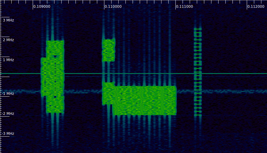
The following Inspectrum waterfall shows the only PDDCH transmission that appears in this recording. It is the one that starts at 0.11 seconds and occupies two disjoint blocks in the frequency domain. The PDSCH transmission of the SIB1 begins immediately after this PDDCH transmission. As we will see in this post, the PDCCH transmission is a DCI format 1_0 that contains the scheduling parameters of the SIB1 PDSCH transmission. The other signals shown in this waterfall are the PBCH/SS block on the left (see the posts about the PBCH and synchronization signals) and a CSI-RS on the right (see the post about reference signals).
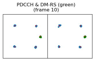
In my post about 5G downlink reference signals, I had already demodulated the PDCCH and wiped off the pseudorandom sequence on its demodulation reference signal, producing the following constellation plot.
Resource elements used by the PDCCH
The first thing that we need to explain is why the PDCCH occupies the set of resource elements that we have seen in this waterfall. In 5G, the PDCCH is transmitted in a CORESET (control resource set). A CORESET designates the resource elements in which the PDCCH can be transmitted. UEs use this knowledge to perform blind decoding of the PDCCH in the CORESET. Since 5G is intended to be very flexible, each cell can use simultaneously different CORESETs, each configured with different parameters. Configuration of the CORESETs is done by the RRC (a higher protocol layer used to configure radio resources), but there is a special CORESET0 that is used to transmit the PDCCH for the SIB1. This exists because when a UE is connecting to a cell, it does not have access to the RRC until it has decoded the SIB1 and it has begun attaching to the cell. Therefore, this special CORESET0 is configured by the MIB, which is transmitted in the PBCH. When a UE connects to a cell, it first synchronizes to the cell and decodes the MIB, obtaining the CORESET0 configuration. Then it listens for PDCCH transmissions in CORESET0, decoding the PDCCH for the SIB1 at some point. After this, it can decode the corresponding SIB1 transmission in the PDSCH.
The MIB parameters that give the CORESET0 configuration are the following.
PDCCH-ConfigSIB1 ::=                SEQUENCE {
    controlResourceSetZero              ControlResourceSetZero,
    searchSpaceZero                     SearchSpaceZero
}

ControlResourceSetZero ::=                  INTEGER (0..15)
SearchSpaceZero ::=                 INTEGER (0..15)
Both fields controlResourceSetZero and searchSpaceZero are indices into tables in Section 13 of TS 38.213 that define the CORESET0 configuration parameters.
In a previous post about the PBCH, we decoded the MIB in this recording, finding the following parameters.
{'message': ('mib',
  {'systemFrameNumber': (b'\xdc', 6),
   'subCarrierSpacingCommon': 'scs15or60',
   'ssb-SubcarrierOffset': 8,
   'dmrs-TypeA-Position': 'pos2',
   'pdcch-ConfigSIB1': {
     'controlResourceSetZero': 0,
     'searchSpaceZero': 0},
   'cellBarred': 'notBarred',
   'intraFreqReselection': 'notAllowed',
   'spare': (b'\x00', 1)})}
Therefore we see that in this cell both controlResourceSetZero and searchSpaceZero are set to zero.
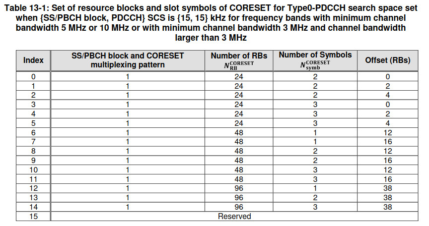
The table that needs to be used with controlResourceSetZero is Table 13-1 in TS 38.213 (the appropriate table depends on the subcarrier spacing and the frequency band). In this table we see that the CORESET0 uses multiplexing pattern 1, it occupies 24 resource blocks and 2 symbols, and has an offset of zero resource blocks.
Another piece of information that we need to use to find where CORESET0 is located in the frequency domain is the ssb-SubcarrierOffset parameter in the MIB. The figure below, taken from this online calculator illustrates how the different parameters are related. The ssb-SubcarrierOffset parameter gives the parameter \(k_{\mathrm{SSB}}\). We must count \(k_{\mathrm{SSB}}\) subcarriers down from the lowest subcarrier of the SS/PBCH block. In this case, \(k_{\mathrm{SSB}} = 8\), as determined in the post about the PBCH (the MSB of \(k_{\mathrm{SSB}}\) is transmitted in an additional bit in the PBCH, not in the MIB).
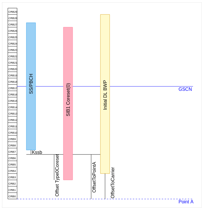
In addition to \(k_{\mathrm{SSB}}\), we also need to count down by as many resource blocks as the offset in the table above indicated. In this case, the offset is zero. This means that CORESET0 starts 8 subcarriers below the lowest subcarrier of the SS/PBCH. I had already commented on this offset in the posts about the PBCH and about the reference signals, since the first subcarrier of CORESET0 needs to be known to generate the appropriate pseudorandom sequence of the PDCCH DM-RS (in the post about the reference signals I computed this offset blindly by cross-correlation).
The table that needs to be used in this case to look up searchSpaceZero is Table 13-11. This table gives the parameters of the monitoring occasions of CORESET0. The UE uses these parameters to determine in which slots it should attempt to decode the PDCCH in CORESET0.
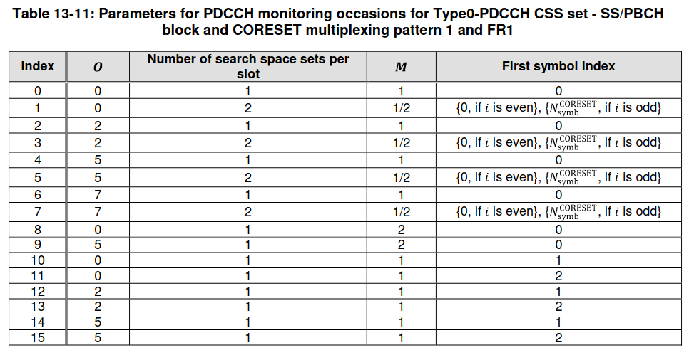
In this analysis the monitoring occasions are not too important, since we have already found visually in the waterfall where the PDCCH transmission happens. Nevertheless, it is good to do the calculations to confirm that everything checks out. Since the searchSpaceZero given in the MIB is zero, the parameters are \(O = 0\), one search space per slot, \(M = 1\), and first symbol index zero.
The monitoring occasions are in slots \(n_0\) and \(n_0 + 1\), where \(n_0\) is computed as \(n_0 = (O \cdot 2^\mu + \lfloor i \cdot M \rfloor) \mod N_{\mathrm{slot}}^{\mathrm{frame},\mu}\). In this formula, \(\mu\) is determined by the subcarrier spacing \(2^\mu \cdot 15\ \mathrm{kHz}\), so \(\mu = 0\) in this case; \(i\) is the SSB index, which is always zero in this recording because only a single SSB is transmitted in each frame; and \(N_{\mathrm{slot}}^{\mathrm{frame},\mu}\) is the number of slots per frame, which is 10 for 15 kHz subcarrier spacing. Therefore, \(n_0 = 0\). Additionally, there is a condition saying that the SFN modulo 2 should be equal to \(\lfloor (O \cdot 2^\mu + \lfloor i \cdot M \rfloor)/N_{\mathrm{slot}}^{\mathrm{frame},\mu}\rfloor \mod 2\). So in this case the monitoring occasions are on even radio frames only.
In this recording, the PDCCH transmissions happens in slot 1 (which corresponds to \(n_0 + 1\)) of a frame with SFN 896 (which is even), so everything checks out. It cannot appear in slot 0 because the PBCH/SS block does not leave enough room.
The next thing we need to explain is why the PDCCH transmission is split into two disjoint blocks in the frequency domain. If we number the resource blocks in CORESET0 as 0, 1, …, 23, we see that this PDCCH transmission occupies resource blocks 3, 4, 5, 6, 7, 8, 15, 16, 17, 18, 19, 20. To explain why this is the case, we need to introduce the concept of CCEs (control channel elements).
A REG (resource element group) is a set of resource elements that occupy one resource block in frequency and one symbol in time. A CCE is a set of 6 REGs. A DCI transmitted in the PDCCH occupies 1, 2, 4, 8 or 16 CCEs. The number of CCEs used by a DCI is known as its aggregation level. The aggregation level indirectly determines the coding rate of the DCI, depending on the DCI size. CCEs are mapped to REGs in a way which is defined in Section 7.3.2.2 of TS 38.211. This section says that REGs are bundled in groups of \(L\) (typically \(L = 6\)) by numbering the resource elements in the CORESET in increasing order of first time and then frequency, and grouping according to this order. Since CORESET0 in this recording has 2 symbols, this means that each REG bundle of \(L = 6\) REGs is formed by 3 resource blocks times 2 symbols.
A permutation maps CCEs to these REG bundles. The permutation depends on several parameters, such as \(L\), \(R\), \(n_{\mathrm{shift}}\) and whether the mapping is interleaved. Generally these parameters are configured by higher layers, but for CORESET0 they are statically defined as \(L = 6\), \(R = 2\), \(n_{\mathrm{shift}} = N_{\mathrm{ID}}^{\mathrm{cell}}\) and interleaved mapping. In this recording we have already found that \(N_{\mathrm{ID}}^{\mathrm{cell}} = 1\). We can enter all these parameters in this online calculator to obtain a diagram that shows how CCEs are mapped to REGs.
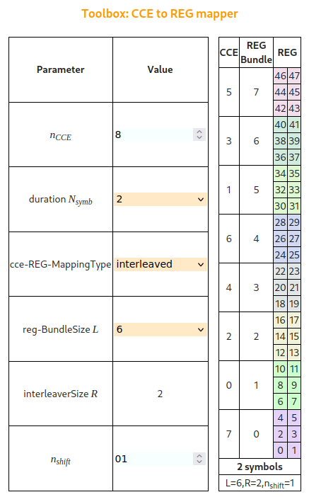
We can see that the PDCCH transmission occupies CCEs 0, 2, 1, 3, which are the first 4 consecutive CCEs. Therefore, it has aggregation level 4. It is split into two distinct blocks in the frequency domain because of the interleaved mapping from CCEs to REG bundles.
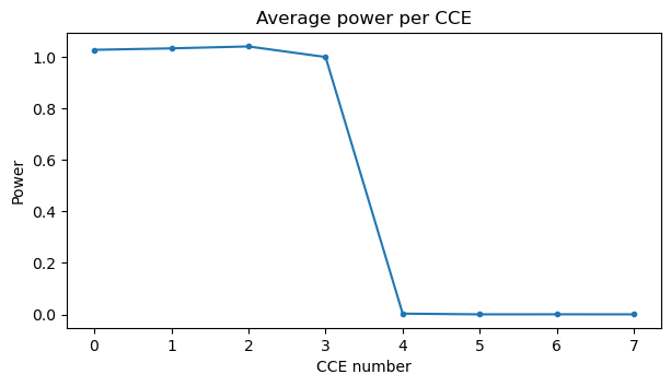
The following plot shows the average power in each CCE in CORESET0. It has been computed by applying the required CCE to REG bundle permutation. In this plot we can also see that the transmission occupies the first 4 CCEs. In more complicated cases we could use this plot to try to figure out how many DCIs are being transmitted in the PDCCH, in the same way that I used plots of RMS amplitude per CCE in my post about the LTE PDCCH.
PDCCH encoding
The channel coding of the PDCCH is quite similar to the PBCH, which I treated in a previous post, since both are based on a Polar code. The main difference is that the PBCH has a message of a single fixed size, while the PDCCH needs to support DCIs of several different sizes. The PDCCH channel coding is described in TS 38.212 Sections 7.3.2 – 7.3.4.
First, a CRC-24 is attached to the DCI. The algorithm is the same as the one used for the PBCH, but there are two differences. One difference is that, for the PDCCH, the CRC register is initialized to all ones, while for the PBCH it is initialized for all zeros. The reason for this is that if the CRC register is initialized to all zeros, then adding zeros to the beginning of a message does not change its CRC. This is not a problem for the PBCH, because the message size is fixed and known by the UE. However it is a problem for blind decoding of the PDCCH, since the UE does not know the DCI size in advance, and it might mistake the DCI for one of a different size if it obtains a valid CRC check when attempting to use the wrong size.
The second difference is that the last 16 bits of the CRC are scrambled by XOR-ing with the RNTI. This is the same as in LTE, and it is used to allow the UE to filter DCIs addressed to it. An interesting difference with LTE is that in LTE the PDCCH CRC is a CRC-16. In my post about about the LTE PDCCH, since I didn’t know which RNTIs were being used, I had to use some heuristics to determine if my decodes were correct. In 5G, the 8 MSBs of the CRC are not scrambled, so it is possible to use them as a weak check of the correctness of a DCI decode, even if the RNTI is not known.
After a CRC-24 is attached to the DCI, the message is encoded with a Polar code. The DCI size plays a role in the configuration of the Polar code parameters. First, the message size \(K\), which is equal to the DCI length plus the 24 bits of the CRC, and the size of the rate matching output \(E\), which is determined by the aggregation level, since each CCE contains 108 bits of PDCCH data (9 QPSK data resource elements per REG, times 6 REGs per CCE), are used together with some formulas in Section 5.3.1 of TS 38.212 to choose \(n\), which determines the Polar code size \(N = 2^n\). This choice of \(n\) is required to satisfy \(n \leq n_{\mathrm{max}} = 9\).
Before Polar coding, the \(K\) bit message is interleaved in the same way as the PBCH, by using a permutation formed by shortening a 164-element permutation.
As for the PBCH, the \(N\)-bit Polar code is extracted from a 1024-bit Polar code. Likewise, the PDCCH uses no parity check bits in the construction of the code: \(n_{\mathrm{PC}} = n_{\mathrm{PC}}^w = 0\). However, there is a difference in the definition of the information bits and frozen bits. This involves the rate matching algorithm, and it is given in Section 5.4.1.1 in TS 38.212. The rate matching algorithm has an \(N\)-bit input and needs to generate an \(E\)-bit output. It considers the following possible cases:
- \(N \leq E\). Then the rate matching algorithm performs extension by repetition. This is the case used for the PBCH, since \(N = 512\) and \(E = 864\). The information bits are defined as the \(K\) most reliable bits of the Polar code.
- \(N > E\) and \(K/E \leq 7/16\). Then the rate matching algorithm performs puncturing by removing the first \(N – E\) bits of the Polar codeword after applying sub-block interleaving. All the bits that get punctured are forced to be in the frozen set. Additionally, bits \(0, 1, \ldots, M – 1\) are also forced to be in the frozen set, where \(M = \lceil 3N/4 – E/2\rceil\) if \(E \geq 3N/4\) or \(M = \lceil 9N/16 – E/4\rceil\) otherwise. The information bits are defined as the \(K\) most reliable bits among the remaining set.
- \(N > E\) and \(K/E > 7/16\). Then the rate matching algorithm performs shortening by removing the last \(N – E\) bits of the Polar codeword after applying sub-block interleaving. All the bits that get punctured are forced to be in the frozen set. The information bits are defined as the \(K\) most reliable bits among the remaining set.
In many cases the additional restrictions that force some bits to be in the frozen set are vacuous, since these bits are already among the \(N – K\) least reliable bits, and so they would be frozen regardless of these additional rules.
Once the set of information and frozen bits are chosen according to these rules, Polar coding is done in the same way as for the PBCH. After Polar coding, sub-block interleaving is also done in the same way as for the PBCH, by dividing the \(N\)-bit Polar codeword into 32 blocks of \(N/32\) bits, and permuting these blocks.
Finally, the \(N\)-bit codeword is rate matched to \(E\) bits as has been described above. If \(N \leq E\), repetition coding is performed by circularly looping over the \(N\)-bit codeword as many times as needed to obtain \(E\) bits. If \(N > E\) and \(K/E \leq 7/16\), then the first \(N – E\) bits are punctured. If \(N > E\) and \(K/E > 7/16\), then the last \(N – E\) bits are removed.
The remaining steps in the PDCCH encoding are described in Section 7.3.2 in TS 38.211. The \(E\)-bit rate matched word is scrambled by XORing with an \(E\)-bit pseudorandom sequence. This pseudorandom sequence is generated using the initialization value \(c_{\mathrm{init}} = (n_{\mathrm{RNTI}} \cdot 2^{16} + n_{\mathrm{ID}}) \mod 2^{31}\). Here \(n_{\mathrm{ID}}\) is typically the cell ID, but it can be set to a different value by higher layers, and \(n_{\mathrm{RNTI}}\) can be optionally set to the C-RNTI by higher layers, but is typically zero. In the case of the PDCCH for the SIB1, \(c_{\mathrm{init}}\) is simply the cell ID.
This scrambled sequence is modulated with QPSK and mapped to the PDCCH data resource elements. Subcarriers with index equal to 1 modulo 4 are reserved for the PDCCH DM-RS. The remaining subcarriers are used for data. The set of resource elements used for this DCI is determined as explained in the previous section by taking into account the REGs corresponding to the CCEs occupied by the DCI. Once the set of resource elements is determined, the QPSK symbols are mapped into these resource elements in increasing order of first frequency and then time. This is something very important that is not mentioned explicitly in the TS and can cause confusion. The definition of CCEs involves a certain ordering and permutation of REGs. This ordering and permutation are only used to define the CCEs. The data is always mapped in increasing order of first frequency and then time into the resource elements occupied by the DCI.
Blind PDCCH sniffing
In my post about the LTE PDCCH, I performed blind sniffing of the PDCCH, by using certain heuristics to detect which CCEs were used and what were the DCI sizes. This process is more difficult than the blind decoding that a UE performs because the UE has some information about what CCEs to monitor and what DCI sizes and RNTIs to expect, so it can try a reasonable number of possible combinations. In a sniffing case, the set of all possible combinations is probably too large. In LTE, there is no good way to validate a correct decoding without the knowledge of the RNTI, and in 5G only 8 bits of the CRC are usable without knowledge of the RNTI, which gives a rather weak validity check.
In this post the situation is quite simple, because there is only one PDCCH transmission and we already know that it is the scheduling for the SIB1. However, here I will give some indications about how to proceed in a more general situation where we have a recording of the downlink of a gNB in which there can be any kind of traffic. Another source of ideas can be this 5G sniffer that performs PDCCH sniffing, but I haven’t looked at their approach in detail.
The DCI size plays a rather important role, because it determines the Polar code size. However, most DCIs are relatively small. Indeed, the largest possible DCI size is 140 bits, which together with the 24 bit CRC, gives \(K = 164\), which is the maximum length supported by the Polar code interleaver.
The mapping of CCEs to DCIs can be obtained by plotting the average amplitude of each CCE and using some guesswork, as I did for LTE. In this case we have seen that there are 4 consecutive CCEs in use, so there is probably a single DCI with an aggregation level of 4. This gives us \(E = 432\).
From the knowledge of \(E\), we can determine the Polar code size \(N = 2^n\) by looking at how the choices in Section 5.3.1 in TS 38.212 work even if we don’t know \(K\) exactly. First we need to check whether \(E \leq (9/8)\cdot 2^{\lceil \log_2 E \rceil – 1}\). This is false for each \(E = 108 \cdot 2^A\), \(k = 0, \ldots, 4\), which are the possible values of \(E\) depending on the aggregation level \(2^A\). Therefore \(n_1 = \lceil \log_2 E\rceil\).
According to Section 7.3.1 in TS 38.212, the minimum DCI size is 12 bits. If a DCI is shorter than this, it is zero extended to 12 bits. Therefore, \(K \geq 36\). This means that \(n_2 = \lceil \log_2 (K/R_{\mathrm{min}})\rceil\) where \(R_{\mathrm{min}}\) satisfies \(n_2 \geq 9\). Therefore, we can simplify \(\min\{n_1, n_2, n_{\mathrm{max}}\} = \min\{n_1, n_{\mathrm{max}}\}\), because \(n_{\mathrm{max}} = 9\). Since \(E \geq 108\), we have \(n_1 = \lceil \log_2 E\rceil \geq 7\). Therefore, the expression \(\max\{\min\{n_1, n_2, n_{\mathrm{max}}\}, n_{\mathrm{min}}\}\) can be simplified to \(\min\{n_1, n_{\mathrm{max}}\}\), because \(n_{\mathrm{min}} = 5\).
So we see that for aggregation level \(2^A\), the Polar code size is determined by \(n = \min\{\lceil \log_2 (108\cdot 2^A)\rceil, 9\}\). This formula gives \(n = 7\) for \(A = 0\), \(n = 8\) for \(A = 1\), and \(n = 9\) for \(A \geq 2\). In particular, in our case \(A = 2\), so \(n = 9\).
The next thing that we need to guess is what rate matching case is used. We know \(E\) and \(N\), as these only depend on the aggregation level \(2^A\), but we do not know \(K\). We can see that \(N \leq E\) if and only if \(A \geq 3\). These large aggregation levels must use repetition coding, since the maximum Polar code size used for the PDCCH is 512.
Something that is useful to compute is \(\lfloor 7E/16 \rfloor\), since whether \(K\) is smaller or greater than this value determines the cut between puncturing and shortening. This gives 47, 94, and 189 for \(A = 0, 1, 2\) respectively. Therefore, in most cases \(K \leq \lfloor 7E/16\rfloor\), and puncturing will be used. In fact, for \(A = 2\), puncturing is always used, since \(K \leq 164\). For \(A = 0, 1\) we might need to consider both puncturing and shortening depending on whether we suspect that the DCI might be large enough to cause shortening.
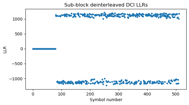
In our case we know that puncturing is the only possible option, because \(A = 2\). First we collect the PDCCH data symbols from the 4 CCEs that are occupied, descramble them, and compute the LLRs of the \(E = 432\) bits. The result is shown here.
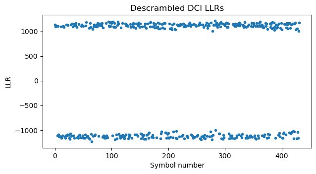
Puncturing is undone by prepending \(N – E = 80\) zeros to these LLRs. Then we undo sub-block interleaving. The sub-block size is \(N/32 = 16\) bits, so the 80 zeros we have added comprise the first 5 sub-blocks. The effect of sub-block interleaving on these first 5 sub-blocks is just to swap blocks 3 and 4. So after sub-block deinterleaving we still find that the first 80 LLRs are zero.
Now we need to perform Polar decoding. For this we need to guess \(K\), since it is used to determine the set of frozen bits. Note that the set of frozen bits decreases as \(K\) increases: if \(K_1 \leq K_2\), then the set of frozen bits for \(K_1\) contains the set of frozen bits for \(K_2\). Denote by \(\hat{K}\) a guess we make, and by \(K\) the true information word length. If \(\hat{K} < K\), then Polar decoding can fail, because some of the information bits that have the value one might lie in the frozen set for \(\hat{K}\), so the decoder will force the value of these bits to be zero, causing more errors in other bits. If \(\hat{K} > K\), then generally decoding will work correctly. We are simply making the decoder’s job more difficult by “forgetting” that some bits are frozen, and having the decoder figure out that they are zero. If the SNR is good, such as in this case, decoding will still succeed.
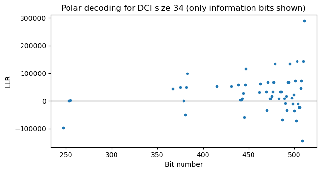
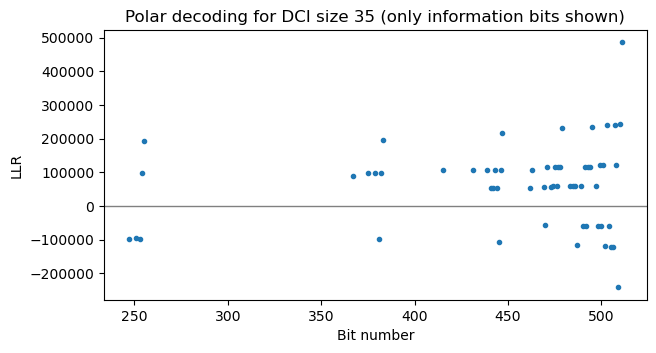
The following two plots compare the LLR output of the Polar decoder assuming DCI sizes of 34 and 35 respectively (so \(\hat{K}\) is 58 and 59 respectively). For a DCI size of 34, there are some LLRs which are very close to zero. This means that decoding has failed, because 34 was smaller than the true DCI size. In contrast, for DCI size 35 all the LLRs are away from zero.
We can use this to our advantage to define a metric that is the minimum absolute value of the output LLRs. If we compute this metric for different values of \(\hat{K}\), we will see that it jumps from a small value to a large value at some particular \(\hat{K}_0\), which in this case is 59 (DCI size 35). This \(\hat{K}_0\) might not be equal to \(K\), because if the \(b\) least reliable bits of the information word are zero, then Polar decoding will succeed if we use \(\hat{K} = K – b\). But at least we know that \(\hat{K}_0 \leq K\) and that \(K – \hat{K}_0\) is generally small.
What we can do now is to continue decoding with \(\hat{K}_0\) and check the CRC-24. If we know the RNTI, then we can check the full CRC-24. If we don’t know the RNTI, then we can still use the 8 MSBs as a check. If we get a wrong CRC, we try with \(\hat{K}_0 + 1\) instead. We continue incrementing our guess \(\hat{K}_0 + j\) in this way until we obtain a CRC match.
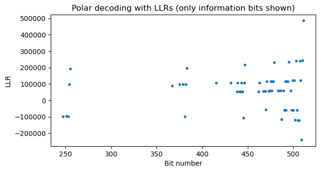
Applying this procedure to the PDCCH in this recording shows that the correct DCI size is 37 rather than 35. We have only needed to check the CRC 3 times in this case: for DCI sizes 35, 36, 37. Therefore, even using the 8 MSBs would give a reasonably low false positive rate. The Polar decoder output LLRs for the correct codeword size \(K = 37 + 24 = 61\) are shown here.
After performing Polar decoding, we deinterleave the \(K\)-bit information word. Then we can compute the CRC of the first \(K-24\) bits. I already had a CRC-24 function implemented for the PBCH, but it performed the calculation byte by byte. In the PDCCH the message size is not a multiple of 8 bits in general, so I have implemented a bit by bit CRC-24 function. This function also needs to initialize the register to 0xffffff, unlike for the PBCH.
After computing this CRC-24, we can check its 8 MSBs against the 8 MSBs of the CRC-24 field in the message. In this case we also know that the DCI has the SI-RNTI, which is 0xffff, so we can XOR the 16 LSBs of the CRC-24 with the SI-RNTI and check them too. The check is successful, which means that the DCI has been decoded correctly.
DCI parsing
In my post about the LTE PDCCH, I used a very useful LTE DCI online decoder to parse the DCIs that I decoded. I haven’t found something equivalent for 5G, so I have written some code to parse the DCI. The contents of each DCI format are defined in Section 7.3.1. To parse a DCI, we need to know its format. In this case we expect the format to be format 1_0, which corresponds to scheduling of PDSCH in one cell. This is the simplest format for PDSCH scheduling, so it makes sense that this is the one used for the SIB1 transmission. In many cases, the DCI format can also be inferred from the DCI size, since different DCI formats often have different sizes.
The size of a particular DCI format typically depends on some of the configuration parameters of the cell, because they affect the size of some fields. For instance, the size any field which speaks about frequency allocations will typically depend on the cell bandwidth. The definition of format 1_0 is in Section 7.3.1.2.1. The fields are slightly different depending on some factors, including the RNTI. So we need to make sure that we are looking at the definition for the SI-RNTI, which is shown here.
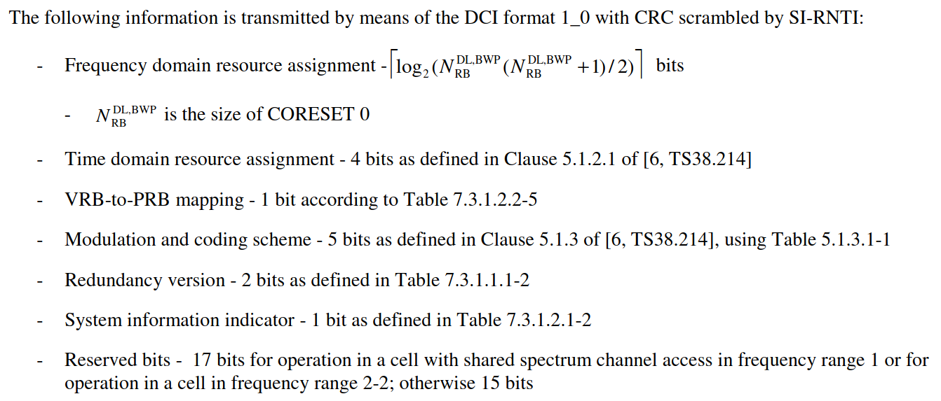
The size of the first field depends on the size of CORESET0. We have \(N_{\mathrm{RB}}^{\mathrm{DL,BWP}} = 24\) in this case, so the size of the frequency domain resource assignment field is 9 bits. The remaining fields are fixed size (the reserved bits field has 15 bits, since this cell is in FR1 and does not use shared spectrum channel access). By summing up the sizes of all the fields, we see that the DCI size is 37 bits. We could have used this knowledge to decode directly the DCI in the previous section, but it is good to have an approach that works in a more general setting.
The values of the fields of this DCI are the following
freq_domain_assign = 168
time_domain_assign = 0
vrb_to_prb_mapping = 0
mcs = 5
rv = 0
system_information_indicator = 0
rsvd = [0 0 0 0 0 0 0 0 0 0 0 0 0 0 0]
The value of the frequency domain resource assignment field needs to be decomposed as indicated in Section 5.1.2.2.2 of TS 38.214. This describes the downlink resource allocation type 1, which is the one used in DCI formats 1_0, 4_0 and 4_1 according to Section 5.1.2.2 in this TS. This allocation type encodes a contiguous set of \(L_{\mathrm{RBs}}\) resource blocks starting at resource block \(RB_{\mathrm{start}}\) as the following \(RIV\) (resource indicator value):\[RIV = \begin{cases}N_{\mathrm{BWP}}^{\mathrm{size}}(L_{\mathrm{RBs}}-1) + RB_{\mathrm{start}} & \mathrm{if}\ L_{\mathrm{RBs}}-1 \leq \lfloor N_{\mathrm{BWP}}^{\mathrm{size}} \rfloor\\ N_{\mathrm{BWP}}^{\mathrm{size}}(N_{\mathrm{BWP}}^{\mathrm{size}} – L_{\mathrm{RBs}} + 1) + N_{\mathrm{BWP}}^{\mathrm{size}} – 1 – RB_{\mathrm{start}} & \mathrm{otherwise}\end{cases}\]
To decode the \(RIV\), note that in both cases it has the form \(RIV = a N_{\mathrm{BWP}}^{\mathrm{size}} + b\) with \(0 \leq a \leq \lfloor N_{\mathrm{BWP}}^{\mathrm{size}} / 2 \rfloor\) and \(0 \leq b < N_{\mathrm{BWP}}^{\mathrm{size}}\). Therefore, we can obtain \(a = \lfloor RIV/N_{\mathrm{BWP}}^{\mathrm{size}}\rfloor\), and \(b = RIV \mod N_{\mathrm{BWP}}^{\mathrm{size}}\). To distinguish between the two cases, we can now compute \(a + b + 1\). In the first case this gives\[a + b + 1 = L_{\mathrm{RBs}} + RB_{\mathrm{start}} \leq N_{\mathrm{BWP}}^{\mathrm{size}}.\]In the second case it gives\[a + b + 1 = 2 N_{\mathrm{BWP}}^{\mathrm{size}} – (L_{\mathrm{RBs}} + RB_{\mathrm{start}}) + 1 \geq N_{\mathrm{BWP}}^{\mathrm{size}} + 1.\]So we see that the first case happens if and only if\[a + b + 1 \leq N_{\mathrm{BWP}}^{\mathrm{size}}.\]
In our case, \(RIV = 168\) and \(N_{\mathrm{BWP}}^{\mathrm{size}} = 24\). Applying this procedure we see that we are in the first case and that \(L_{\mathrm{RBs}} = 8\), and \(RB_{\mathrm{start}} = 0\). This means that the PDSCH transmission occupies the lowest 8 resource blocks of the bandwidth part corresponding to CORESET0. This matches what we see in the waterfall of the recording.
To interpret the time domain resource assignment field we need to go first to Table 5.1.2.1.1.-1 in TS 38.214 to find that the applicable table for SI-RNTI in the Type0 common PDCCH search space with SS/PBCH block and CORESET multiplexing pattern 1 uses the table for Default A for normal CP. This table is Table 5.1.2.1.1-2, shown here.
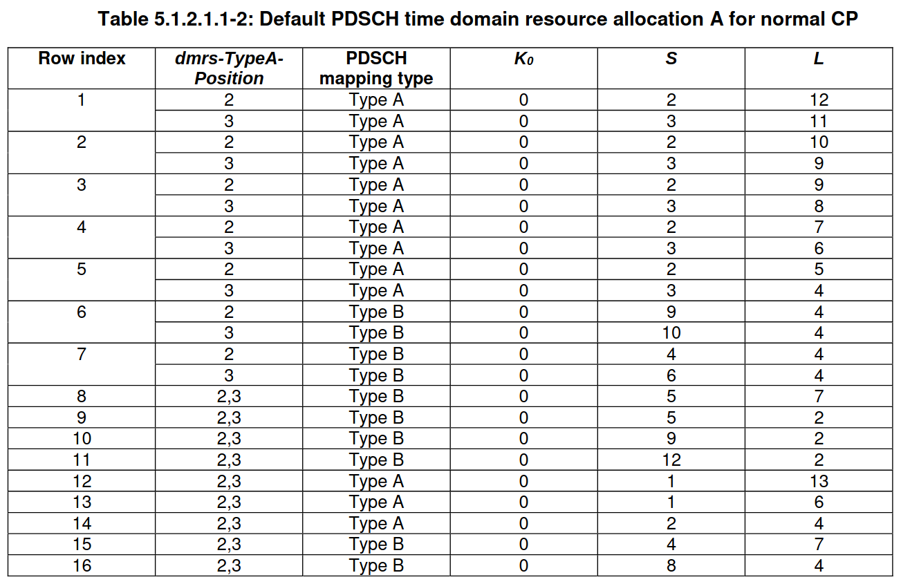
The row index of this table corresponds to the value of the time domain resource assignment field plus one. In this case, the field contains the value zero, so we must use row index 1. The MIB contains the value of dmrs-TypeA-Position, which is 2 in this case, as we saw in the post about the PBCH. So we see that the parameters that we need to use are \(K_0 = 0\), \(S = 2\), \(L = 12\).
The parameter \(K_0\) is the slot offset. Simplifying some of the formulas in Section 5.1.2.1 for this particular case, we see that the slot allocated to the PDSCH is \(K_s = n + K_0\), where \(n\) is the slot containing the DCI. Therefore, in this case the PDSCH is transmitted in the same slot as the DCI, as we have seen in the waterfall.
The parameter \(S\) is the start symbol of the PDSCH. In this case it starts in symbol 2, right after the PDSCH, which occupies the first two symbols of the slot. The parameter \(L\) is the allocation length. In this case, \(L = 12\), which means that the PDSCH occupies the remaining 12 symbols of the 14-symbol slot.
The VRB to PRB mapping field contains the value zero, which means that the mapping is non-interleaved.
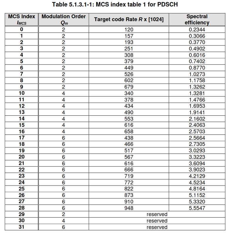
The MCS field has the value 5. The applicable table for DCI format 1_0 with SI-RNTI is Table 5.1.3.1-1 in TS 38.214, shown here. The index 5 corresponds to QPSK modulation with a target coding rate of 0.37. This is a reasonable configuration to allow the SIB1 to be decoded even in low SNR conditions.
The redundancy version field has the value zero. This is used in FEC decoding of the PDSCH. The system information indicator field is zero. This means that the PDSCH transmission is for the SIB1 (instead of a SI message), as we expected. All the 15 reserved bits are zero.
Code and data
As usual, all the calculations and plots in this post are done in this Jupyter notebook. The SigMF recording can be found here.
One comment