Decoding BGM-1 GMSK telemetry

In my previous post, I analyzed the Doppler of the Blue Ghost Mission 1 S-band telemetry signal during its lunar landing. The mission came to an end on March 16, as night fell on the landing site. During the 14 days that it has been operating on the lunar surface, BGM-1 has been transmitting low-rate GMSK telemetry on S-band at some times, and a high-rate signal on X-band at other times (this is said to be up to 10 Mbps DVB-S2), including some periods of no transmissions, presumably for thermal management.

In this post I will show how to decode the GMSK S-band telemetry signal with GNU Radio. I will use the IQ recording done by CAMRAS with the Dwingeloo 25 m radiotelescope during the landing as an example, since this dataset is publicly available.

The signal is 15360 baud GMSK, with the usual precoder that allows coherent demodulation as OQPSK (see Figure 2.4.17A-1 in the Radio Frequency and Modulation Systems CCSDS Blue Book). The coding is CCSDS concatenated coding with a Reed-Solomon interleaving depth of 4. The frame size is 892 bytes (4 times 223). The frames are CCSDS TM Space Data Link frames, but there is a bug in how the Reed-Solomon interleaving is implemented. The contents of the Space Data Link frames are encrypted, probably using CCSDS SDLS.

Laurent decomposition of GMSK

As part of this post, I wanted to make a reasonably good GNU Radio GMSK coherent demodulator flowgraph using the Laurent decomposition that is presented in the paper Exact and Approximate Construction of Digital Phase Modulations by Superposition of Amplitude Modulated Pulses (AMP). This is an old paper from the 80s, but it contains the theory of the relation between MSK modulations and OQPSK in a self-contained and clean way.

The paper treats a somewhat more general case, but here I will summarize the results for the particular case of pulse-shaped MSK. Denote the symbol duration by \(T\) and assume that we have a pulse shape function \(p(t)\) such that \(p(t) = 0\) for \(t < 0\) and for \(t > LT\), where \(L\) is a suitable chosen integer, and that furthermore \(p(t)\) is normalized so that\[\int_{-\infty}^{+\infty} p(t)\, dt = \frac{\pi}{2}.\]We put\[\varphi(t) = \int_{-\infty}^t p(s)\, ds\]and define the pulse-shaped MSK waveform by\[x(t) = \exp\left(i\sum_{n\in\mathbb{Z}} a_n \varphi(t – nT)\right),\]where \(a_n \in \{1, -1\}\) are binary symbols.

GMSK is a particular case of pulse-shaped MSK. In GMSK, a Gaussian kernel\[h(t) = B \sqrt{\frac{2\pi}{\log 2}} \exp\left(-\frac{2\pi^2B^2t^2}{\log 2}\right)\]is defined. The constant outside of the exponential normalizes the kernel to have an integral of one. The constant multiplying \(t^2\) inside the exponential is chosen so that \(B\) is the 3 dB one-sided bandwidth of this kernel. More in detail, if\[H(f) = \int_{-\infty}^{+\infty} h(t) e^{-2\pi i ft}\, dt\]is the Fourier transform of \(h(t)\) (which is also a Gaussian), then\[H(B) = \frac{\sqrt{2}}{2} H(0).\]

The bandwidth \(B\) is defined in terms of the dimensionless quantity \(BT\), which commonly ranges between 0.25 and 1. The Gaussian kernel is convolved with a rectangular pulse of duration \(T\) (also normalized to integral one): \(r(t) = 1/T\) for \(|t| \leq T/2\), and \(r(t) = 0\) elsewhere. This yields the pulse shape\[q(t) = (r \ast h)(t) = \frac{1}{T}\int_{-T/2}^{T/2}h(t – s)\, ds.\]Note that\[\int_{-\infty}^{+\infty}q(t)\,dt = 1.\]This pulse shape \(q(t)\) can be written in the form above by choosing \(L\) large enough that\[A = \int_{-LT/2}^{LT/2} q(t)\,dt\]is very close to one, and then setting\[p(t) = \frac{\pi}{2A}q(t – LT/2),\qquad 0\leq t \leq LT.\](This amounts to throwing away the tails of the Gaussian to obtain a pulse of finite duration).

The paper by Laurent shows that this kind of pulse-shaped MSK modulation can be written in an exact way as a PAM waveform using a collection of \(M = 2^{L-1}\) pulse shapes \(C_0(t), \ldots, C_{M-1}(t)\), so that\[x(t) = \sum_{n\in\mathbb{Z}} \sum_{k=0}^{M-1} c_{n,k} C_k(t – nT),\]where the coefficients \(c_{n,k}\) are calculated in terms of the symbols \(a_n\). Usually, the pulses \(C_k(t)\) for \(k \geq 1\) are much smaller than \(C_0(t)\), so they can be ignored to obtain an approximated expression\[x(t) \approx \sum_{n\in\mathbb{Z}} b_n C_0(t-nT),\]where\[b_n = c_{n,0}= i^{\sum_{j=-\infty}^n a_j}.\]The formula for \(b_n\) in terms of \(a_n\) has a straightforward interpretation. The term \(\sum_{j=-\infty}^n a_j\) is just an “integral encoder” of the input bits (this is the inverse of a differential encoder). Raising \(i\) to the output of this integral encoder corresponds to alternating between the real and imaginary part (so alternating between I and Q, as OQPSK does), and changing sign every time two consecutive \(a_n\) are equal. With some calculations it is easy to check that the CCSDS precoder is basically the inverse operation of this transformation from \(a_n\) to \(b_n\). So precoding allows the data to be read directly from the symbols \(b_n\).

The expression above shows that pulse-shaped MSK is approximately equal to an OQPSK modulation with pulse \(C_0(t)\). All that remains is to compute the OQPSK pulse \(C_0(t)\) in terms of the MSK pulse \(p(t)\). To this end, we define \(\Psi(t)\) as \(\Psi(t) = \varphi(t)\) for \(t < LT\) and \(\Psi(t) = \varphi(LT-t)\) for \(t \geq LT\). Note that \(\Psi(t)\) is obtained by reflecting the “phase pulse” \(\varphi(t)\), which goes from 0 to \(\pi/2\), in order to obtain a phase pulse that goes from 0 to \(\pi/2\) and then back to 0. We now put\[S_0(t) = \sin \Phi(t)\]and\[S_n(t) = S_0(t + nT).\]The pulse \(C_0(t)\) is given by\[C_0(t) = \prod_{j=0}^{L-1} S_j(t).\]Since \(S_n(t)\) is zero for \(t\) outside of the interval \([-nT, (2L-n)T]\), we see that \(C_0(t)\) is zero outside of the interval \([0, LT]\).

In the case of a discrete-time GMSK modem, the taps for the MSK pulse \(p[n]\) are usually computed by evaluating the Gaussian kernel \(h(t)\) at the sampling times to discretize it, and then performing the convolution with a discrete-time rectangular pulse \(r[n]\) (assuming an integer number of samples per symbol). The taps for the OQPSK pulse \(C_0[n]\) can be calculated by using the discrete-time equivalent of the formulas given above.

GNU Radio GMSK demodulator

To validate my implementation of a GMSK demodulator based on the Laurent decomposition, I have made a GNU Radio flowgraph that contains a GMSK modulator, a channel model, and the GMSK demodulator. This is shown here.

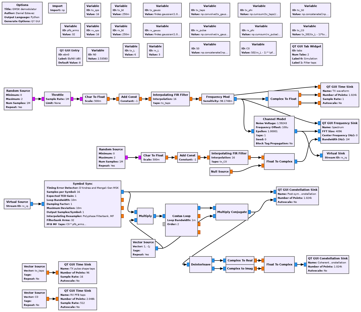
The GMSK modulator works by interpolating the NRZ symbols with an FIR filter constructed by convolving a Gaussian and a rectangular pulse, and then using the Frequency Mod block with the appropriate sensitivity.

The demodulator uses the Symbol Sync block with the “D’Andrea and Mengali Gen MSK” time error detector. This TED appears in the paper A digital approach to clock recovery in generalized minimum shift keying by D’Andrea, Mengali and Reggiannini. Pulse shape filtering is done in the Symbol Sync block with a matched filter polyphase filter bank that has been computed with the Laurent decomposition.

At the output of the Symbol Sync, ignoring carrier phase rotation due to frequency error for a moment, the constellation looks like the following, for \(BT = 1\).

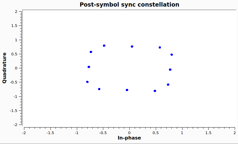
The way to understand this constellation is as follows. At “even” symbols, we are integrating a pulse on the I branch of the OQSK signal. So the real part of the constellation is going to be either +1 or -1. However, we are also integrating the two symbols on the Q branch that straddle this I branch symbol. If those two Q symbols have opposite sign, they cancel out and the imaginary part is zero. However, if they have the same sign, they have a rather large contribution \(\pm i\alpha\) (think of \(\alpha \approx 0.8\)). So the symbol we see is either \(\pm 1\) or \(\pm 1 \pm i \alpha\). In “odd” symbols, we are integrating a pulse on the Q branch of OQPSK signal. An analogous reasoning shows that we either get \(\pm i\) or \(\pm i \pm \alpha\). These are the points that we see in the constellation above. We can think of this constellation as \(\pi/2\)-BPSK with heavy inter-symbol interference.

I have decided to perform carrier phase recovery in the following way. First, “odd” symbols are multiplied by \(-i\) in order to transform \(\pi/2\)-BPSK into regular BPSK. We still have heavy inter-symbol interference, but a BPSK Costas loop is able to lock on the constellation, albeit with reduced performance. After the Costas loop, we undo this multiplication by \(-i\), obtaining again the \(\pi/2\)-BPSK constellation, but now phase-locked. Finally, the real part of each even symbol and the imaginary part from the next symbol are grouped together to form a QPSK symbol.

An alternative approach would be to include the transformation to a QPSK symbol as part of the carrier phase recovery loop. In this approach, the output of the Symbol Sync would first be rotated in phase according to the loop state, then the real part of each even symbol and the imaginary part of the next symbol would be grouped as a complex symbol, a QPSK phase error detector would be applied, and the error would be used to close the loop. I don’t know which of the two approaches is better. This second approach has the advantage that when the loop is locked, the phase error detector does not see the heavy inter-symbol interference. It sees a regular QPSK constellation. However, being a QPSK phase error detector, it has more squaring losses than a BPSK phase error detector. Also, while the loop is closing we have something weird instead of a QPSK constellation, so I don’t know if this approach always closes the loop reliably. Ultimately the reason why I decided to use the first approach is because the second approach needs a custom GNU Radio block, since it is not possible to close a loop that encompasses multiple blocks.

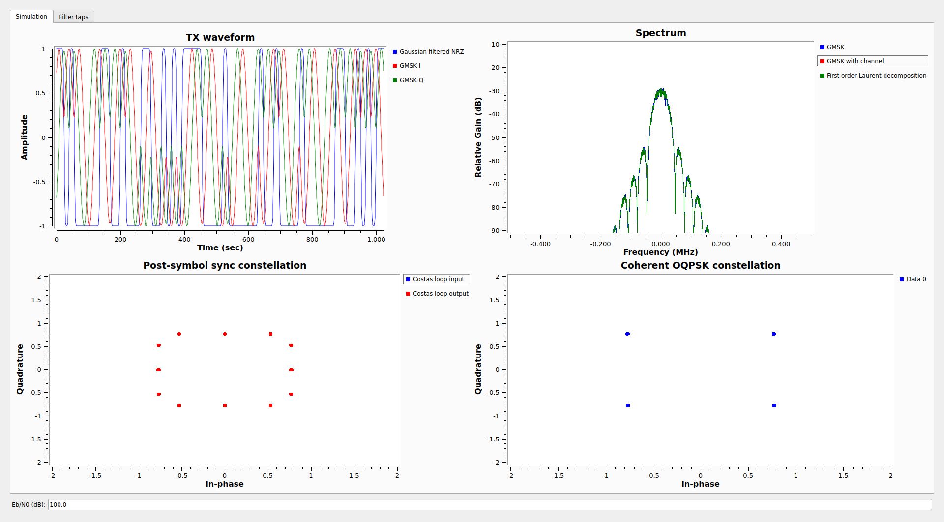
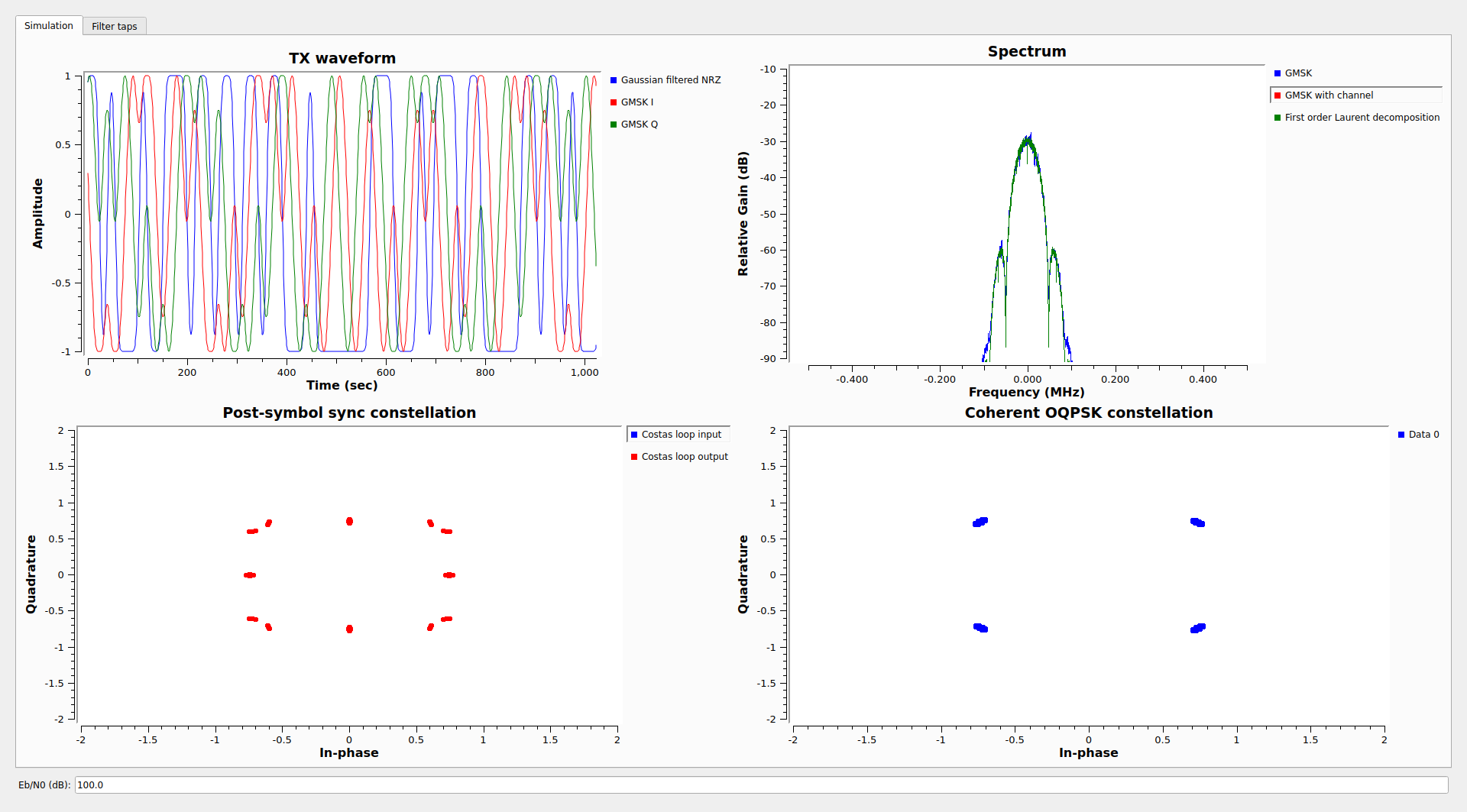
The following shows the GUI of the simulation with very high SNR and \(BT = 1\). To verify that I have computed the Lauren decomposition pulse correctly, I am generating a BPSK signal with random symbols and this pulse shape, and comparing its spectrum to the spectrum of the GMSK signal. The two should be very close unless there are errors in the implementation. In this case we have a very clean OQPSK constellation at the output of the receiver.

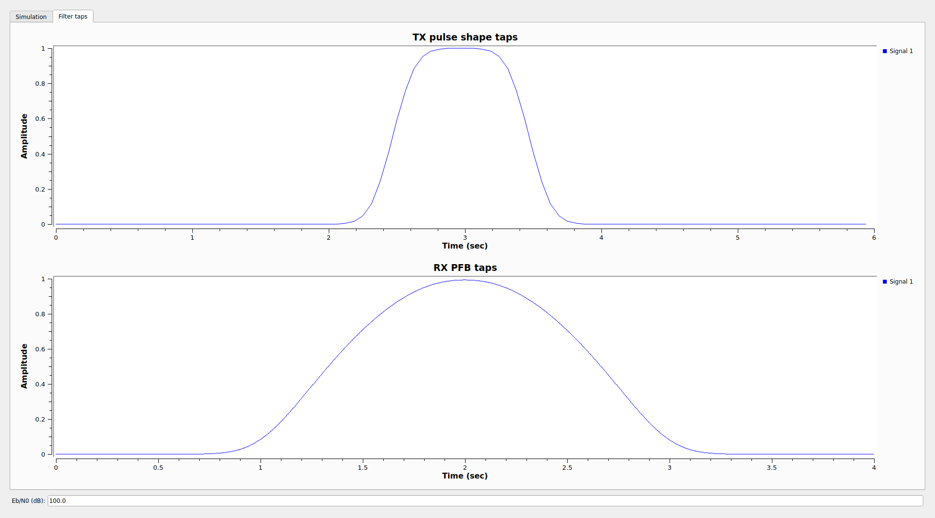
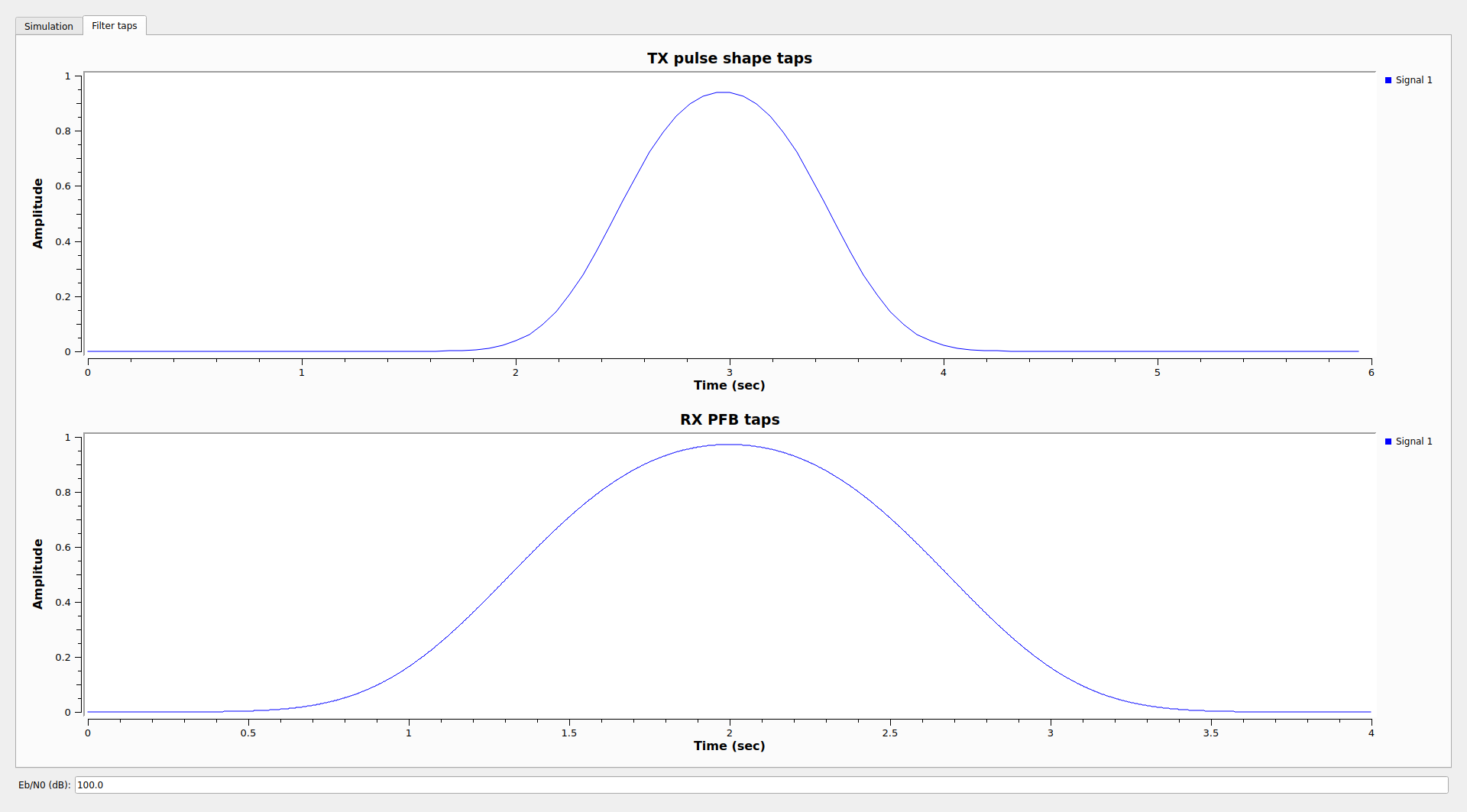
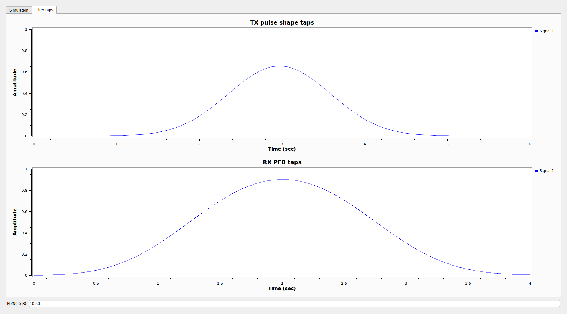
I’m using another tab in the GUI to plot the pulse shapes used in the transmitter (the convolution of a rectangular pulse with a Gaussian kernel) and the receiver (the Laurent decomposition pulse). For comparison, remember that for GMSK with \(BT = \infty\), which is the same as MSK with a rectangular pulse, the Laurent decomposition pulse is a half-sine pulse with a duration of two symbols. Here we see something that looks like a smoothed version of that. The horizontal axis of these plots is in symbols. GNU Radio says “Time (sec)”, and it is not possible to change the label (I could have used a QT GUI Vector Sink instead of a Time Sink).

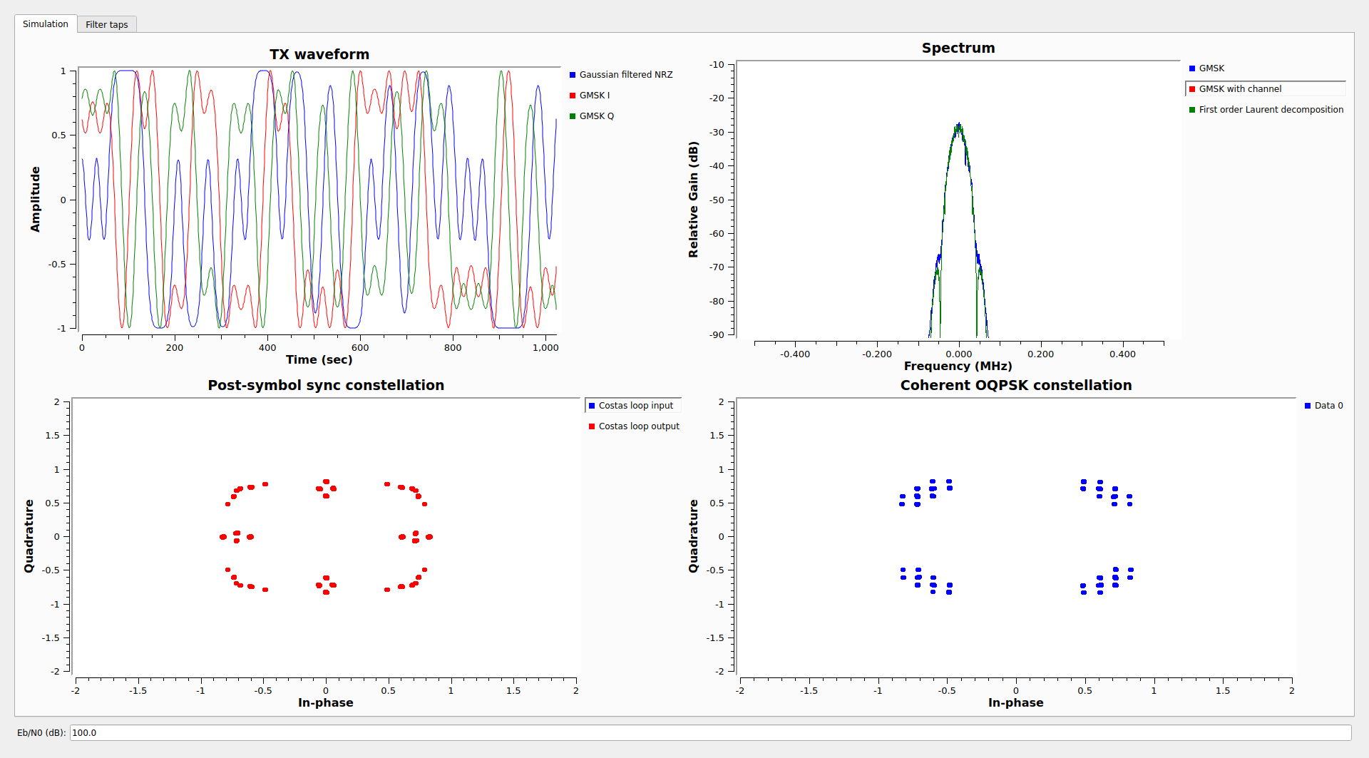
For \(BT = 0.5\) we start getting some inter-symbol interference in the OQPSK constellation. We also see that there is a small difference between the GMSK spectrum and the Laurent pulse spectrum.

For \(BT = 0.25\) the inter-symbol interference is rather large. There is more difference between the GMSK spectrum and the Laurent pulse spectrum, but it is still very minor. The Laurent pulse is still completely valid as a matched filter for the receiver.

The following screenshot shows the operation of the receiver in more typical conditions. The channel model noise is adjusted for an Eb/N0 of 8 dB. The BT is 0.25.

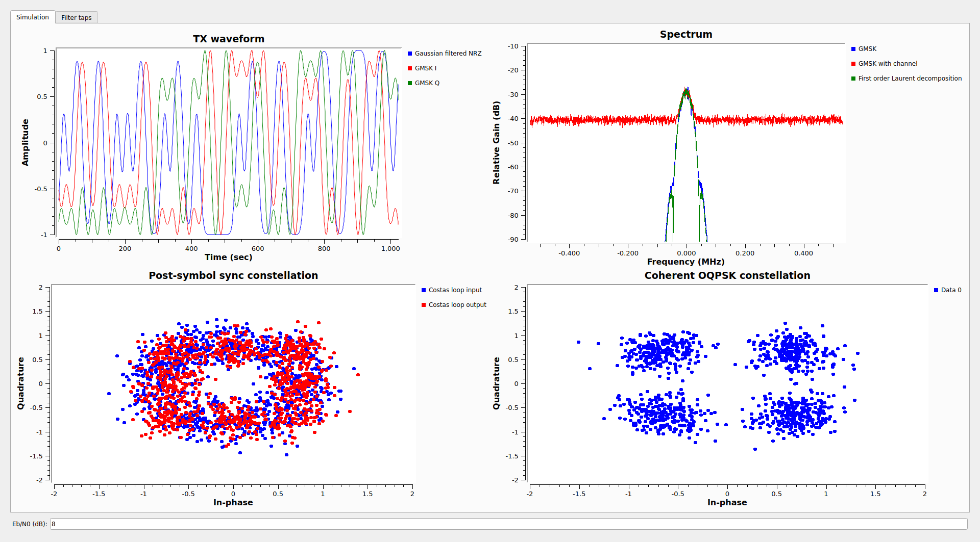
BGM-1 decoder

The GNU Radio flowgraph used to decode the recording from Dwingeloo is shown here. The 4 Msps IQ file is downconverted and decimated by 32, which gives a samples/symbol very close to 8. After that, there is an AGC and the GMSK coherent demodulator shown above.

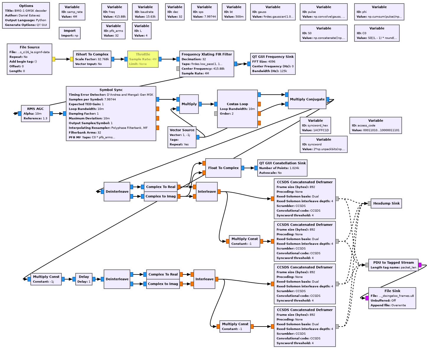
The next step regards handling phase ambiguity. I haven’t touched on this in the previous section, but the OQPSK constellation at the output of the demodulator has 4 possible rotations for phase ambiguity (rotations by multiples of 90 deg). It is not difficult to convince ourselves that no matter how we handle an OQPSK signal, there will be 4 possible ambiguity states (this is basically because of the symmetries that OQPSK has). However, depending on the specific algorithm used, part of this ambiguity might manifest in how to pair up adjacent symbols or it might manifest as a phase ambiguity.

The way in which the ambiguity is handled in this receiver is to do an independent branch (a different phase rotation) for each possible case. In each of the branches, a CCSDS Concatenated Deframer block from gr-satellites performs Viterbi decoding (which internally requires two branches per block, so this could be optimized because the OQPSK constellation has already solved how to pair up convolutional encoder symbols unambiguously), ASM detection and Reed-Solomon decoding. Despite the fact that 8 cases are tried in parallel, Reed-Solomon decoder errors are usually enough to filter out false ASM detections, so the amount of false frames at the output should be really low.

I haven’t measured the \(BT\) of the BGM-1 signal accurately. CCSDS recommends \(BT = 0.25\) for GMSK used by Category A missions , which are near space missions at less than 1 million km from Earth (see footnote 4 in Page 2.4.17A-1 in the Blue Book). However, I have seen that for this recording the constellation looks better when demodulating with \(BT = 0.5\), so this is the value that I’m using in the flowgraph.

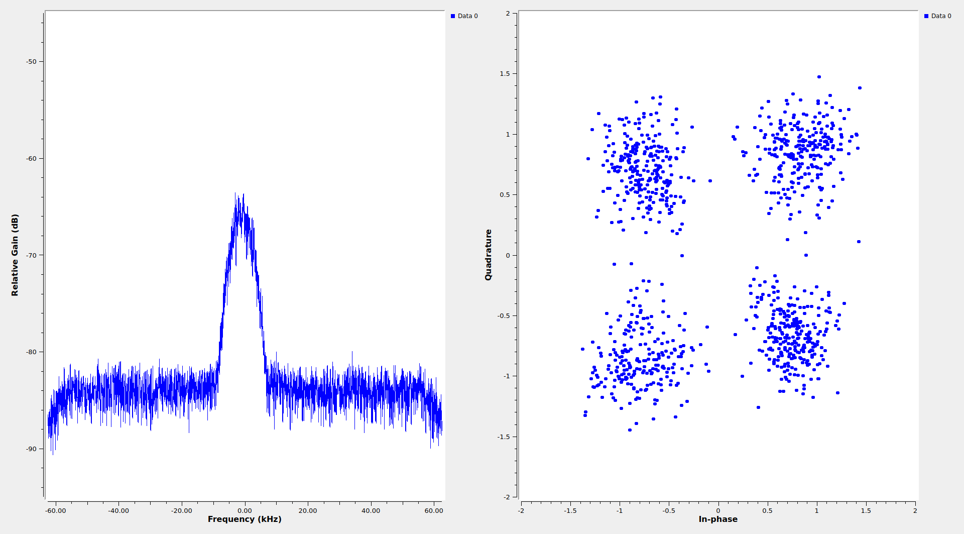
The following screenshot shows the decoder flowgraph running on the Dwingeloo recording. The SNR is quite good, so the constellation has few bit errors.

Reed-Solomon interleaving bug

When I started to analyze the frames, I was quite puzzled, because most of the contents of the frames seemed encrypted (which makes a lot of sense for this mission), but a few fields scattered around the beginning of the frame were unencrypted and I could see some binary counters. I could not find any relation between these and any CCSDS protocol. Eventually, I noticed what was happening. The Reed-Solomon interleaving done by BGM-1 is not implemented as CCSDS specifies.

The details of how Reed-Solomon interleaving should be implemented are described in Section 4.4.1 of the TM Synchronization and Channel Coding Blue Book. Schematically, interleaving works as indicated in this diagram.

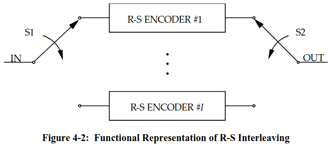
The switches S1 and S2 are commuted for each input and output byte. This means that the first message byte goes to encoder 1, the second goes to encoder 2, etc., while the output is formed by the first output of encoder 1, the first output of encoder 2, and so on in this order. Since each individual Reed-Solomon encoder is systematic, the result is a systematic code too. Said in other words. The message ends up in the output in exactly the same order, followed by all the parity check bytes generated by the encoders.

The decoder works in the same way but in reverse. This is how the Reed-Solomon decoder in gr-satellites is implemented. However, to make sense of the frames I decoded from BGM-1, I found that I had to interleave the frames at the output of the Reed-Solomon decoder. More precisely, I had to write each frame by rows in a matrix with 4 columns and then read it by columns. This means that the Reed-Solomon interleaving in BGM-1 is not correctly implemented (or at least, deviates from what CCSDS recommends).

In terms of the interleaver diagram above, what BGM-1 is actually doing is to feed the first 223 bytes of the message all to encoder 1, the next 223 bytes of the message all to encoder 2, and so on until feeding the last 223 bytes of the message to encoder 4. The first switch is commuted only every 223 bytes. However, the second switch is still commuted for every output byte, so the output is still the first byte from encoder 1, the first byte from encoder 2, and so on (otherwise the gr-satellites Reed-Solomon decoder would have failed to decode these codewords). Note that with this implementation the result is not a systematic code. The message ends up interleaved at the encoder output, which is the reason why I had to interleave it back to its original form after Reed-Solomon decoding.

Telemetry frames

The telemetry frames are CCSDS TM Space Data Link frames. There is an FECF (CRC-16) at the end of each frame. Only 0.38% of the decoded frames have a wrong CRC. This is normal, because the Reed-Solomon decoder has a low probability of claiming successful decoding on a bad frame.

There are two virtual channels in use: virtual channel 2 and virtual channel 7 (which is the only idle data virtual channel). The spacecraft ID is 0x4. I haven’t found an assignment for BGM-1 in the SANA registry.

The master channel frame count and virtual channel frame count do not work in the way that CCSDS specifies. All the idle frames in virtual channel 7 are identical, so their master channel frame count and virtual channel frame count do not increment (they are always both equal to 2, for some reason). The frames in virtual channel 2 always have the same master channel frame count and virtual channel frame count, because idle frames from virtual channel 7 do not increment the master channel frame count.

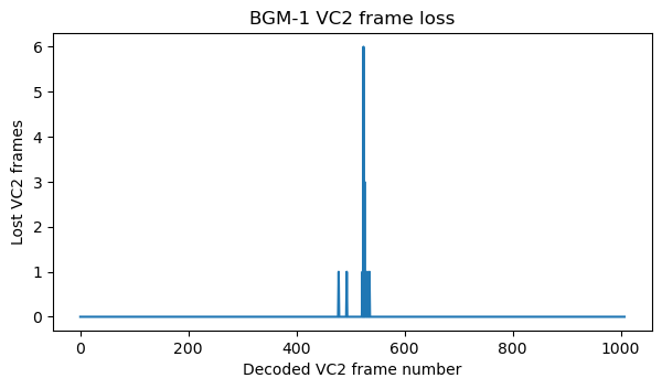
Here is a plot of the frame loss in VC2 computed by looking at discontinuities in the unwrapped virtual channel frame count. There are a few lost frames around the middle of the recording, perhaps because the Doppler rate is larger than what the Costas loop can handle.

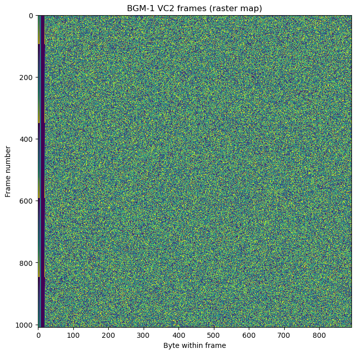
Most of the decoded frames belong to VC2. In VC7 there are only a few frames towards the end of the recording. The contents of the VC2 frames are shown in this raster map. We can see that, except for a few bytes of headers, the data looks random, as expected for encrypted data.

The next raster map shows the first 32 bytes in each VC2 frame.

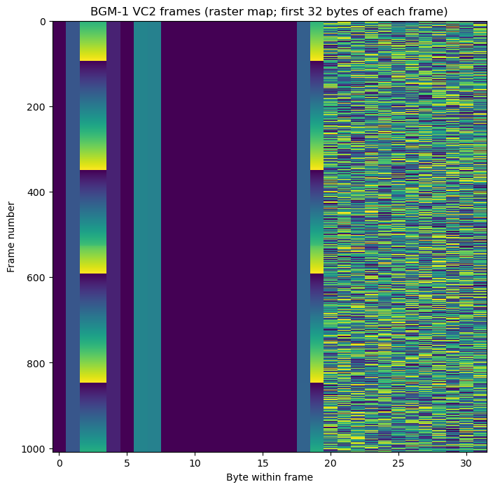
The first 6 bytes are the TM Space Data Link primary header. Then there are 14 bytes before the encrypted data. I believe these are an SDLS Security Header. The first 2 bytes of this header would be the SPI (security parameter index). It is always 0x7370 in these frames. Of the remaining 12 bytes, the first 10 have zeros, and the last 2 are a counter. This 12-byte field could be a sequence number, or perhaps only some of the last bytes are a sequence number, and the rest is an initialization vector which is always zero.

The contents of VC7 idle frames are a bit strange. All these frames are identical, as shown in this raster map.

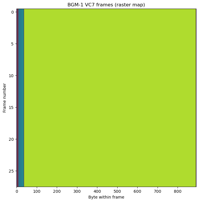
Starting at byte 37, and until reaching the last two bytes (which carry the CRC-16), the payload is always 0xe0. It is quite typical to fill the payload of idle frames with a constant value, although CCSDS now recommends the use of a pseudorandom sequence.

However, the strange part comes between the TM Space Data Link primary header and byte 37, where the 0xe0‘s start. First there is 0xfe00001f. Then there are the letters abcdefghijklmnopqrstuvwxyz in ASCII. Finally, there is 0xa0, which is an ASCII line feed character.

Code and data

The materials used in this post can be found in this repository. This includes the GNU Radio flowgraphs, the Jupyter notebook for telemetry frames analysis, and a binary file with the decoded frames. The IQ recording from Dwingeloo can be downloaded here.