Whenever I implement a PLL or a similar control loop, I invariably consult the formulas in the paper Controlled-Root Formulation for Digital Phase-Locked Loops, by Stephens and Thomas. Other sources that give formulas for the loop coefficients in terms of the loop bandwidth perform a continuous time analysis and then use a bilinear transform or a similar kind of transform to translate results between continuous time and discrete time. The appeal of the paper by Stephens and Thomas is that they work directly in discrete time, using a beautiful complex contour integral argument to calculate the loop bandwidth in terms of the loop coefficients for a loop of any order. Unfortunately, their method doesn’t give a closed-form formula for the loop coefficients in terms of the loop bandwidth. The loop coefficients can be obtained numerically, and the paper gives tables for common loop bandwidths and orders.
In most of my designs I use a second order loop with supercritical damping, which means that the two loop roots in the z-plane are equal (and hence real). As I was doing a design the other day, I wondered whether in this specific situation, which is much simpler than the general case, a closed-form solution could be obtained. It turns out that this is the case, so I’ll be using this formula from now on. In this short post I explain how this is done and give the formula.
I will be using the same notation as in the Stephens and Thomas paper. The loop noise bandwidth is denoted by \(B_L\) and the sampling interval is denoted by \(T\) (in units of Hz and seconds respectively). We work in terms of the normalized loop bandwidth \(B_L T\), which is adimensional. The loop takes as input the \(n\)-th phase measurement of the signal, \(\phi_n\), and uses the \(n\)-th model phase \(\hat{\phi}_n\) calculated by the loop to compute an error \(\tilde{\phi}_n = \phi_n – \hat{\phi}_n\). The model phase update in terms of the error is given by\[\hat{\dot\phi}_{n+1}T = K_1\tilde{\phi}_n + K_2\sum_{i=1}^n \widetilde{\phi}_i,\]where \(K_1\), \(K_2\) are the loop coefficients, and\[\hat{\phi}_{n+1} = \hat{\phi}_n + \hat{\dot\phi}_{n+1}T.\]
The so called loop roots, which are the poles of the closed-loop transfer function, are denoted by \(z_1\), \(z_2\). Section IV E, the paper gives a relation between the elementary symmetric polynomials on the loop roots and the loop coefficients. For a second order loop, this relation is\[\begin{split}z_1 + z_2 &= 2 – K_1 – K_2\\z_1z_2 &= 1 – K_1.\end{split}\]
The loop bandwidth is given in terms of the loop coefficients in Table IV. For a second order loop this is\[B_L T = \frac{2K_1^2 + 2K_2 + K_1K_2}{2K_1(4 – 2K_1 – K_2)}.\]
We will study only the supercritical damping case, where the two loop roots are equal, \(z_1 = z_2 = z = e^{-\beta T}\), for some \(\beta > 0\). Replacing this into the formulas above, we see that\[K_1 = 1 – z^2,\qquad K_2 = (1 – z)^2.\] Now this can be replaced in the formula for the loop bandwidth, obtaining\[B_L T = \frac{(1 – z)(z^2 + 4z + 5)}{2(z+1)^3}.\]
The key remark is that this gives a cubic equation for \(z\) in terms of \(B_L T\). The cubic equation has a solution that, even if somewhat complicated, can be written in closed form using some cubic roots. The cubic equation has three solutions, but we are looking for a solution satisfying \(0 < z < 1\).
We can use Wolfram Alpha or another computer algebra package to obtain this solution. We get\[z = \frac{12 B_L T + 6}{3 \sqrt[3]{6} (2 B_L T + 1) \Delta} + \frac{\sqrt[3]{2} \Delta}{\sqrt[3]{9}(2 B_L T + 1)} – 1,\]where\[\Delta = \sqrt[3]{36 (B_LT)^2 + \sqrt{3}\sqrt{432 (B_LT)^4 + 848 (B_LT)^3 + 624 (B_LT)^2 + 204 B_L T + 25} + 36 B_L T + 9}.\]Once \(z\) is obtained from \(B_L T\) using this formula, the loop coefficients \(K_1 = 1 – z^2\) and \(K_2 = (1-z)^2\) can be calculated.
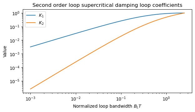
The following plot shows the loop coefficients computed using this formula. Note that the formula is not valid for \(B_L T > 3/2\), because for \(B_L T = 3/2\) it gives \(z = 0\).
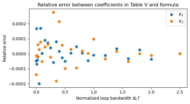
To check the validity of the formula, we compare the filter coefficients given in Table V in the paper with the filter coefficients computed using the formula. The following plot shows the relative error.
These plots have been done in the following Jupyter notebook.
One comment