Two sinusoidal signals are said to be in quadrature if they have a constant phase difference of 90º. Quadrature signals are widely used in signal processing. A digital quadrature oscillator is just an algorithm that computes the sequence \(x_n = (\cos(\omega n), \sin(\omega n))\), \(n\geq 0\), or a similar sequence of sinusoids in quadrature. Here \(\omega\) is the oscillator frequency in radians per sample. Direct computation of this sequence is very time consuming, because the trigonometric functions have to be evaluated for each sample. Therefore, it is a good idea to use a linear recurrence scheme to compute \(x_n\). Using basic trigonometric identities, we see that\[x_{n+1} = A x_n,\quad x_0=\begin{pmatrix}1\\0\end{pmatrix},\]with\[A = \begin{pmatrix}\alpha_1 & -\alpha_2\\\alpha_2 & \alpha_1\end{pmatrix},\quad \alpha_1 = \cos(\omega),\ \alpha_2=\sin(\omega).\]
However, to actually perform these computations in a digital processor, one has to quantize \(\alpha_1,\alpha_2\), meaning that one has to replace \(\alpha_1,\alpha_2\) by approximations. It is easy to see that if one replaces \(\alpha_1,\alpha_2\) by some perturbation, then the eigenvalues of \(A\) are no longer in the unit circle, so the oscillation can grow or decay exponentially and one would need to apply an AGC scheme to keep this method stable.
Here we will look at a new quadrature oscillator by Martin Vicanek that has appeared recently and solves this problem.
Vicanek’s idea starts by considering the oscillator \(y_n\) for frequency \(\omega/2\). We write \(y_{n+1} = B y_n\), where \(B\) is defined as \(A\) but replacing \(\alpha_1\) by \(\beta_1 = \cos(\omega/2)\) and \(\alpha_2\) by \(\beta_2 = \sin(\omega/2)\). We note that \(x_n = y_{2n}\), so that if we denote by \(x_{n+1} = A_\beta x_n\) the recurrence for the original oscillator of frequency \(\omega\), then \(A_\beta = B^2\). Performing the computation, we see that\[A_\beta = \begin{pmatrix}\beta_1^2-\beta_2^2 & -2\beta_1\beta_2\\2\beta_1\beta_2 & \beta_1^2-\beta_2^2\end{pmatrix}.\]
Vicanek goes on and rewrites the matrix \(A_\beta\) as\[A_k = \begin{pmatrix}1-k_1k_2 & -2k_1+k_1^2k_2\\k_2 & 1-k_1k_2\end{pmatrix},\]where\[\quad k_1 = \tan(\omega/2),\ k_2 = \sin(\omega)=2k_1/(1+k_1^2).\]Actually, this rewriting allows him to reduce the number of multiplications to just 3 (instead of the usual 4) when computing \(x_{n+1}\) from \(x_n\), but it is also critical for the performance of the method.
Of course, these matrices \(A\), \(A_\beta\) and \(A_k\) are the same, but what happens when one perturbs \(k_1,k_2\) is different from what happens when one perturbs \(\alpha_1,\alpha_2\) or \(\beta_1,\beta_2\). When studying the stability of these methods, we note that the point where more precision is lost is when computing trigonometric functions. Therefore, we assume on our analysis that \(\alpha_1,\alpha_2,\beta_1,\beta_2,k_1,k_2\) are just approximations and that the rest of the operations can be computed exactly.
We will look at real Toeplitz matrices of the form \[T = \begin{pmatrix}a & b\\c & a\end{pmatrix}\] and see whether the recurrence \(x_{n+1}=T x_n\) gives something that can be useful as a quadrature oscillator. A general \(2\times 2\) matrix can be studied in a similar way, but the calculations become more cumbersome. The first condition is that the eigenvalues of \(T\) have to be in the unit circle, because if not, the recurrence will grow or decay exponentially. Moreover, the eigenvalues cannot be real, because this would only give trivial oscillators with \(\omega\) an integer multiple of \(\pi\). The characteristic polynomial of \(T\) is\[p(\lambda)=\lambda^2-2a\lambda+a^2-bc.\] Since its zeros are complex conjugates and lie in the unit circle, their product must be 1, so we have \[a^2 – bc = 1.\]
Now we see that the matrices \(A\) and \(A_\beta\) do not satisfy this condition for general values of \(\alpha_1,\alpha_2,\beta_1,\beta_2\). However, \(A_k\) satisfies this condition for every \(k_1,k_2\).
The zeros of \(p\) are non-real if and only if its discriminant is negative. Since \(a^2-bc=1\), this is equivalent to \(|a|<1\). For the matrix \(A_k\), this translates to the condition \(|1-k_1k_2| < 1\), which will satisfied as long as \(k_1,k_2\) are good approximations, since for their exact values \(1-k_1k_2 = \cos(\omega)\). Moreover, if one computes \(k_2\) as \(k_2=2k_1/(1+k_1^2)\), then \(1-k_1k_2 = (1-k_1^2)/(1+k_1^2)\), which has modulus smaller than \(1\) as long as \(k_1\neq 0\).
We denote by \(e^{i\nu}\) and \(e^{-i\nu}\) the zeros of \(p\). By looking at the coefficient of \(\lambda\) in \(p\), we see that \(a = \cos\nu\). Let \(v=(v_1,v_2)\) be a (complex) eigenvector such that \(Tv = e^{i\nu} v\). This equality implies that\[iv_1\sin \nu = b v_2.\] Since \(a^2-bc=1\) and \(|a|<1\), we see that \(b\neq 0\), so that \(v_1 \neq 0\), because \(v \neq 0\). Multiplying \(v\) by a suitable scalar, we may assume \(v_1 = 1\), so that\[v = \begin{pmatrix}1\\ -i\tau\end{pmatrix},\quad \tau = -\frac{\sin\nu}{b}.\](The \(-\) sign is just for aesthetic reasons in the latter).
Put \(w = \overline{v} = (1,i\tau)\). Since \(T\) is real, we have \(T^nv = e^{in\nu}v\) and \(T^n w = e^{-in\nu}w\). Adding these two equalities and dividing by \(2\), we get\[\tag{1}T^n\begin{pmatrix}1 \\ 0\end{pmatrix} = \begin{pmatrix}\cos(n\nu) \\ \tau\sin(n\nu)\end{pmatrix}.\]This implies that the recurrence \(x_{n+1} = T x_n\) with \(x_0 = (1,0)\) gives a quadrature oscillator, because the components of \(x_n\) are sinusoids with a constant phase difference of 90º. Similar calculations show that for any initial \(x_0\), the recurrence \(x_{n+1} = T x_n\) will also give two sinusoids with a constant phase difference of 90º and amplitudes related by a factor of \(\tau\), so the choice of \(x_0 = (1,0)\) is not important.
The amplitudes of these two sinusoids are the same if and only if \(\tau=\pm1\), this is, when \(b = \mp \sin \nu\). In this case, \(a^2-bc=1\) implies that \(c = -b\), so \(T\) is just the matrix of the rotation of angle \(\pm \nu\). This is really no surprise, because the equality (1) for \(n=0,1\) already defines \(T\) uniquely, since the vectors \((1,0)\) and \((\cos\nu,\tau\sin\nu)\) are linearly independent.
In summary, when \(a=\cos\omega\), \(c=-b=\sin\omega\), we get \(\nu = \omega\) and \(\tau = 1\), as we expected. When \(a,b,c\) are just approximations to these values, then \(\nu\) is approximately \(\omega\) and \(\tau\) is approximately \(1\).
For many applications, it is important that the amplitudes of the two components of the quadrature oscillator are the same. For instance, if this oscillator is used in a heterodyne mixer, the mixer will exhibit image frequency response if the amplitudes of the two components of the oscillator are not the same. For other applications, this may not be so important. For instance, if the oscillator is used to perform QAM, then a mismatch in the amplitudes will just cause some stretching in the constellation pattern.
In Vicanek’s oscillator, if \(k_2\) is computed as \(k_2 = 2k_1/(1+k_1^2)\), then it is easy to check that \(b=-c\), so that it will have \(|\tau| = 1\) for whatever choice of \(k_1\). Therefore, it is a good idea to compute \(k_2\) in this way and not as \(k_2 = \sin \omega\), not only to avoid the computation of the trigonometric function, but to ensure that the amplitudes are well matched.
This analysis shows that Vicanek’s recurrence \(x_{n+1}=A_k x_n\), indeed gives a quadrature oscillator of frequency approximately \(\omega\) and amplitudes 1 when \(k_1\) is approximately \(\tan(\omega/2)\) and \(k_2 = 2k_1/(1+k_1^2)\).
We have seen that, to give a good quadrature oscillator, the matrix \(T\) should be a rotation matrix\[\tag{2}T = \begin{pmatrix}\cos\nu & -\sin\nu\\\sin\nu & \cos\nu\end{pmatrix},\] even when the parameters that define \(T\) are perturbed. In the case of Vicanek’s oscillator, using the trigonometric identities\[\cos\omega = \frac{1-\tan^2\frac{\omega}{2}}{1+\tan^2\frac{\omega}{2}},\quad\sin\omega=\frac{2\tan\frac{\omega}{2}}{1+\tan^2\frac{\omega}{2}},\] we see that \(A_k\) has the appropriate form when \(k_2\) is computed in terms of \(k_1\), because\[A_k = \frac{1}{1+k_1^2}\begin{pmatrix}1-k_1^2 & -2k_1\\ 2k_1 & 1-k_1^2\end{pmatrix}.\]
One independent way to arrive at this formula for \(A_k\) is as follows. Since we know that \(T\) has to be a rotation matrix as in (2), we want to find real rational functions \(f,g\in\mathbb{R}(t)\) such that \(f^2 + g^2 = 1\). Then we put \(a=f(t)\) and \(c=-b=g(t)\), so that \(a=\cos\nu\), \(c=\sin\nu\) for some \(\nu=\nu(t)\). However, we see that such pair \(f,g\) is just a rational parametrization of the algebraic curve \(x^2 + y^2 = 1\), so we are led to the usual choice \(f(t) = (1-t^2)/(1+t^2)\), \(g(t) = 2t/(1+t^2)\).
Another nice thing about Vicanek’s oscillator is that it is defined in terms of the tangent function, which satisfies a simple first order differential equation. This implies that if one is doing frequency modulation of the oscillator and the deviation \(\Delta \omega\) is small, then we may approximate the deviation of the parameter \(k_1\) as\[\Delta k_1 \approx \frac{dk_1}{d\omega}\Delta\omega = \frac{1}{2}\left(1+\tan^2\frac{\omega}{2}\right)\Delta\omega = \frac{1}{2}(1+k_1^2)\Delta\omega.\] Using this approximation, it is not necessary to compute trigonometric functions when the frequency gets updated.
How does Vicanek’s oscillator actually perform in numerical simulations? Well, I must say that the results of my tests have been very good.
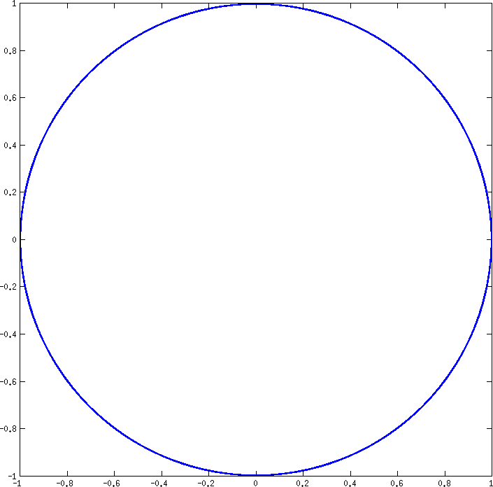
In one of the tests, I start with \(\omega=0.01\) (about 70.19Hz at 44100Hz) and run the oscillator for \(10^9\) samples (6 hours at 44100Hz). When computing \(k_1\), I introduce a random absolute error of size \(10^{-5}\), and I also introduce an absolute error of \(10^{-6}\) in the rest of the computations (including the recursion update). Finally, I take the last \(10^7\) samples to analyse. The XY plot of these \(10^7\) samples shows that the oscillator maintains a constant amplitude of 1 quite well.
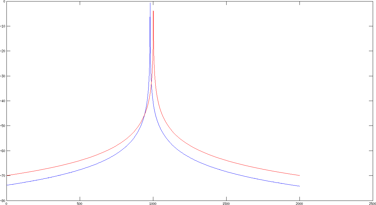
I also compute the FFT of the \(10^7\) samples and plot it in dB with the normalization that the constant signal 1 should be 0dB. The plot of Vicanek’s oscillator is in blue. The plot in red corresponds to an oscillator computed by evaluating the trigonometric functions at each sample, just for comparison. The first plot shows 2000 bins around the frequency of the oscillator. We can see that the oscillator is slightly wrong in frequency, due to the error on the computation of \(k_1\). However, the error in frequency is actually only 1.35e-5 radians/sample (0.07Hz at 44100Hz). Clearly we are to expect this kind of error with an error of \(10^{-5}\) in \(k_1\). We can also see that the phase noise performance of the oscillator is very good.
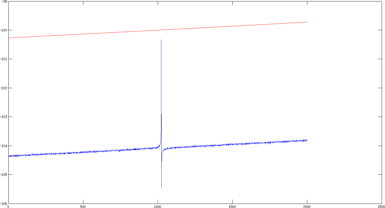
The second plot shows 2000 bins around the image frequency of the oscillator. The image frequency is just a term for \(-\omega\), and the response of the oscillator at this frequency shows to which degree the two components’ phases fail to be in quadrature or their amplitudes fail to match. We can see a spike in the response, mainly due to the error in the computation of \(k_2\), but the image response is 100dB down, which is really good.
I have put the MATLAB code for these computations in Gist. I have also played with the parameters, trying different frequencies and errors (also relative error instead of absolute error). As long as the error in each step of the computations is not very large (around \(10^{-6}\) is OK in many cases), the oscillator will be stable in frequency and the phase noise will be very good. One can also allow a fairly large error in the computation of \(k_2\), although the image response will not be very good if the error is large. Finally, an error in \(k_1\) will just cause an error in frequency of comparable magnitude.
One comment