On matched filtering in the presence of carrier frequency offset

If \(\{x_k\}_{k=0}^{N-1}\) is a complex waveform and this waveform is received in AWGN, that is, the sequence \(y_k = A x_k + n_k\) is received, where \(A\) is an unknown complex amplitude and \(n_k\) are independent circularly symmetric normal random variables with standard deviation one, it is well known that the linear filter \(\{a_k\}_{k=0}^{N-1}\) that maximizes the detection SNR of \(T = \sum_{k=0}^{N-1} a_k y_k\), which is defined as \(|\mathbb{E}[T]|^2/V(T)\), is given by the matched filter \(a_k = \overline{x_k}\).

A natural question is what happens if the waveform is received with an unknown carrier frequency offset \(f\). That is, if \(y_k = A e^{2\pi i f k} x_k + n_k\). The typical solution is to use a bank of matched filters which are spaced by \(\Delta\) in the frequency domain and cover the expected carrier frequency offset range. This means that we use filters \(a_{k,m} = e^{-2\pi i \Delta m k} \overline{x_k}\), where the integers \(m\) are such that the grid of frequencies \(\Delta m\) covers the required frequency range. Here the hope is that if \(\Delta\) is small enough, then choosing the integer \(m\) such that \(\Delta m\) is closest to \(f\), we have that\[T = \sum_{k=0}^{N-1} e^{-2\pi i \Delta m k} \overline{x_k}y_k = A \sum_{k=0}^{N-1} e^{2 \pi i (f-\Delta m) k} |x_k|^2 + \sum_{k=0}^{N-1} e^{-2 \pi i \Delta m k} \overline{x_k} n_k.\]If \(\Delta m-f\) is small, this expression will have an SNR similar to the SNR for \(f = 0\).

However it is possible to do better. We can modify the matched filter to improve the SNR when there is frequency error. Since we choose the filter \(m\) from the bank such that \(\Delta m\) is closest to \(f\), we can assume that \(|f| \leq \Delta / 2\) and that we choose bank \(m = 0\). Now we can pose an optimization problem that involves the frequency error \(f\). Different kinds of optimization problems will lead to different solutions. A natural quantity to maximize is the average SNR with respect to \(f\), assuming that \(f\) is uniformly distributed in \([-\frac{\Delta}{2},\frac{\Delta}{2}]\). This is\[\frac{1}{\Delta}\int_{-\frac{\Delta}{2}}^{\frac{\Delta}{2}} \frac{|\mathbb{E}[T]|^2}{V(T)}\, df.\]Let us solve the optimization problem.

Similarly to the case of the matched filter with no frequency error, we have\[\mathbb{E}[T] = A \sum_{k=0}^{N-1} e^{2 \pi i f k} a_k x_k,\]so\[V(T) = \mathbb{E}[|T-\mathbb{E}[T]|^2] = \mathbb{E}\left[\left|\sum_{k=0}^{N-1} a_k n_k\right|^2\right] = \sum_{k = 0}^{N-1} |a_k|^2.\]Therefore, the optimization problem is equivalent to finding a vector \(\{a_k\}_{k=0}^{N-1}\) with unit norm (\(\sum_{k=0}^{N-1} |a_k|^2 = 1\)) that maximizes the expression\[\frac{1}{\Delta}\int_{-\frac{\Delta}{2}}^{\frac{\Delta}{2}}\left|\sum_{k=0}^{N-1} e^{2\pi i f k} a_k x_k\right|^2\, df.\]This expression can be rewritten as\[\frac{1}{\Delta}\sum_{k=0}^{N-1}\sum_{l=0}^{N-1}\overline{a_l x_l}a_k x_k \int_{-\frac{\Delta}{2}}^{\frac{\Delta}{2}} e^{2\pi i f (k-l)}\, df = \sum_{k=0}^{N-1}\sum_{l=0}^{N-1}\overline{a_l x_l}a_k x_k \operatorname{sinc} (\Delta (k-l)),\]where \(\operatorname{sinc}(x) = \sin(\pi x)/(\pi x)\).

Write \(x_k = e^{i\theta_k}|x_k|\) and denote by \(G\) the matrix with entries \(G_{kl} = |x_k||x_l|\operatorname{sinc} (\Delta (k-l))\). This matrix is the Gram matrix of the vectors \(\varphi_k(f) = e^{2 \pi i f k}|x_k|\) in \(L^2[-\frac{\Delta}{2}, \frac{\Delta}{2}]\) (with the Lebesgue measure multiplied by the normalization factor \(\frac{1}{\Delta}\)), so it is positive semidefinite (and it is positive definite if \(\Delta > 0\) and \(x_k \neq 0\) for all \(k = 0, \ldots, N-1\)). Let \(u = \{u_k\}_{k=0}^{N-1}\) be any unit norm eigenvector corresponding to the largest eigenvalue of \(G\). The solution to the optimization problem is then given by \(a_k = e^{-i\theta_k} u_k\).

The case in which \(|x_k| = 1\) for all \(k = 0, \ldots, N-1\) is particularly important, because it corresponds to constant-envelope modulations, and it is also easier to treat than the general case. This case includes the case of detecting a CW carrier, which corresponds to \(x_k = 1\) for all \(k\). In this case, the Gram matrix \(G\) is simply a matrix of sinc functions \(G_{kl} = \operatorname{sinc} (\Delta (k-l))\). This matrix has been studied by Slepian in 1978, because it appears in the spectral concentration problem, which is equivalent to the optimization problem I’m presenting here. In the spectral concentration problem we consider a unit norm sequence \(\{a_k\}_{k=0}^{N-1}\) and its Fourier transform\[U(f) = \sum_{k=0}^{N-1} e^{-2\pi i f k}a_k.\]The energy that \(\{a_k\}\) has in the frequency band \([-\frac{\Delta}{2}, \frac{\Delta}{2}]\) is\[\int_{-\frac{\Delta}{2}}^{\frac{\Delta}{2}} |U(f)|^2\,df.\]The problem asks which unit norm sequences \(\{a_k\}\) maximize the energy in this frequency band. It is clear that this is equivalent to a particular case of the optimization problem that we are considering (the case \(x_k = 1\) for all \(k\)).

The eigenvectors of the matrix \(G\) given by \(G_{kl} = \operatorname{sinc} (\Delta (k-l))\) can be computed numerically, but the problem is ill-conditioned for large \(N\), because many eigenvalues cluster around the largest eigenvalue. There is a trick to compute the eigenvectors without running into issues. In our case, we can use that trick to compute the eigenvector corresponding to the largest eigenvalue. The trick starts by noticing that the tridiagonal symmetric matrix \(R\) defined by\[\begin{split}R_{k,k} &= \cos(\pi\Delta) \left(k-\frac{N-1}{2}\right)^2,\ k = 0,\ldots, N-1\\R_{k,k+1} = R_{k+1,k} &= \frac{1}{2}(k+1)(N-1-k),\qquad k = 0,\ldots,N-2\end{split}\]commutes with \(G\) (this is shown by some straightforward calculations). This implies that the eigenspaces of \(G\) and \(R\) are the same. All the eigenvalues of a tridiagonal matrix with non-zero entries in its upper diagonal are simple. This is because the first component of an eigenvector for a given eigenvalue determines the remaining components (this is a very simple calculation). Moreover, it is also possible to prove that if \(v_0, v_1, \ldots, v_{N-1}\) are the eigenvectors of \(R\) with corresponding eigenvalues \(\lambda_0 > \lambda_1 > \cdots > \lambda_{N-1}\), then \(v_0, v_1, \ldots, v_{N-1}\) (which must be eigenvectors of \(G\)) have eigenvalues \(\mu_0 > \mu_1 > \cdots > \mu_{N-1}\) as eigenvectors of \(G\). However I haven’t been able to find a reference that proves this in a straightforward way, though presumably this follows from all the calculations in Slepian’s paper. This means that the eigenvector \(u\) that we need can be computed as \(v_0\), the eigenvector corresponding to the largest eigenvalue \(\lambda_0\) of \(R\).

There are efficient algorithms to compute eigenvalues and eigenvectors for tridiagonal symmetric matrices. For instance, SciPy has an eigh_tridiagonal function. Additionally it is possible to use these algorithms to compute only a selection of some of the eigenvalues and eigenvectors. This is precisely what we need, because in our case we only want the eigenvector \(v_0\) corresponding to the largest eigenvalue \(\lambda_0\) of \(R\).

The eigenvectors \(v_0, v_1, \ldots, v_{N-1}\) are called discrete prolate spheroidal sequences (DPSS) and they also play a role in other similar spectral concentration problems and in multitaper spectral analysis. They can be calculated with the dpss window function in SciPy. The first DPSS, also known as Slepian window, and \(v_0\) in our eigenvector notation, is the vector that solves our optimization problem in the constant-envelope case. That is, when \(|x_k| = 1\) for all \(k = 0, \ldots, N-1\). The takeaway of this post is:

In the general case in which the waveform is not constant-envelope, the trick of using a tridiagonal matrix does not work, and we can also have ill-conditioning when trying to compute the eigenvectors numerically (for instance by using the eigh SciPy function).

It is convenient to put the above theoretical results in perspective and show what they really imply for the usual practical applications. In most applications \(\Delta \lesssim 1/N\). For instance, when an FFT is used to detect a CW carrier, we have \(\Delta = 1/N\), because in this case \(\Delta\) is equal to the FFT bin spacing. Other matched filter applications that use an FFT similarly set \(\Delta\) in relation to the FFT bin spacing.

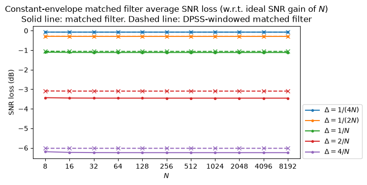
The following plot shows, for a constant-envelope waveform of \(N\) samples, what is the average SNR loss when there is a carrier frequency offset \(f\) uniformly distributed on \([-\frac{\Delta}{2},\frac{\Delta}{2}]\), for both the matched filter (solid lines) and for a matched filter weighted with the DPSS window (dashed lines). The values of \(\Delta = 1/(4N)\), \(1/(2N)\), \(1/N\), \(2/N\), \(4/N\) are shown. We see that there is almost no dependence on \(N\), which is to be expected because this problem can be approximated well by an analogous continuous-time problem. We also see that for the smallest values of \(\Delta\) the loss of the matched filter is already quite small and the DPSS weighting gives almost no improvement.

Since the behaviour changes very little with \(N\), it is better to study what happens for a fixed \(N\) (here \(N = 8192\)), in terms of \(\Delta N\). This is what the plot below shows.

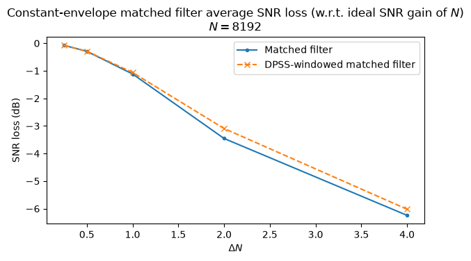
Another good takeaway from this plot is:

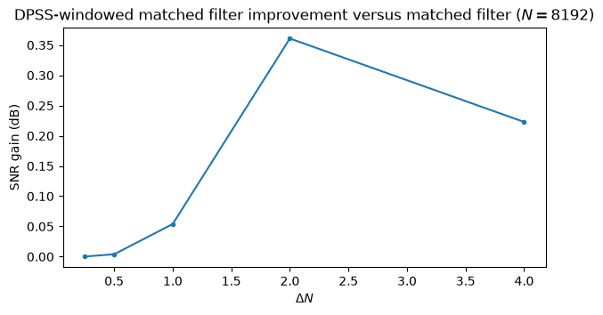
The following figure shows the difference between the two traces in the figure above. This indicates how much improvement is obtained by applying DPSS weighting to the matched filter. For \(\Delta = 1/N\) the improvement is 0.05 dB, which explains why this is rarely done in practice. However for \(\Delta = 2/N\) the improvement is 0.36 dB, so DPSS weighting can be a useful technique if we need to implement a system that is in this situation for whatever reason. Note that interestingly the improvement decreases for \(\Delta > 2/N\).

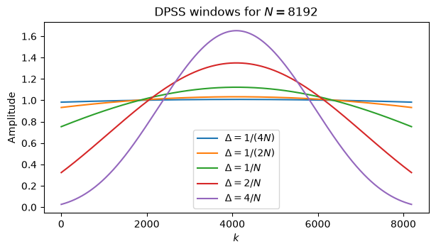
Finally, the following plot shows the DPSS windows. As expected, when \(\Delta\) decreases they tend to a rectangular window, and as \(\Delta\) increases the window tapers off more.

These plots have been made in this Jupyter notebook.

Here I have treated the optimization of the average SNR assuming a uniform distribution of \(f \in [-\frac{\Delta}{2},\frac{\Delta}{2}]\). An equally interesting and useful optimization criterion is to maximize the worst-case SNR. That is, find the sequence \(\{a_k\}\) with unit norm that maximizes\[\min_{|f| \leq \frac{\Delta}{2}}\frac{|\mathbb{E}[T]|^2}{V(T)} = \min_{|f| \leq \frac{\Delta}{2}} \left|\sum_{k=0}^{N-1} e^{2\pi i f k} a_k x_k\right|^2.\]The techniques that are applicable in this problem are related to the Remez exchange used for optimal FIR design, but since the solution is quite involved, this might be a topic for another time.